Assignment 4, CSC 101
Parts 1 and 2 due February 11, 11:59pmParts 3, 4, and 5 due February 20, 11:59pm
This assignment pulls together the work of the previous assignments to create a functional (though somewhat hard-coded) ray casting program. In order to do so you will need to provide a few more data definitions and implement some functions (two required, but likely a few more as helper functions).
Unlike the previous assignments, your solution to this assignment will be built up in parts.
Files
Create a hw4 directory in which to develop your solution. You will also need to copy your files from the previous assignment. Since the solution to this assignment is developed in parts, you may also choose to create subdirectories corresponding to each part.
You will develop the new parts of your program solution over three files. You must use the specified names for your files.
cast.py- contains the function implementationstests.py- contains your test cases for individual functions (unit tests)casting_test.py- contains a main function and a scene cast test (system test)
Once you are ready to do so, and you may choose to do so often while incrementally developing your solution, run your test cases with the command python tests.py. To run your system test (to generate an image) use the command python casting_test.py > image.ppm.
A Note on Color
The concept of a color appears in two different manifestations in this
assignment. The majority of your code will work with a color as represented
by red, green, and blue components that are float values.
While, technically, such components should only range from 0.0 to 1.0, some of
the arithmetic on colors (in the later parts) will allow for values greater
than 1.0 (this is due to an "intensity" scaling factor).
The other representation of a color is strictly for the output format that is used in this assignment (the ppm P3 format discussed here). This representation requires integer values strictly in the range [0, 255] (for our purposes).
Converting between different representations is something that is often
done in programming. For this assignment, all of your calculations
are to be done in terms of float values.
Then, just prior to printing, scale the color components so that they fall
into the range [0, 255] (capping the values at 255), convert to an integer,
and then print the components (you can write a separate utility function for
converting).
Part 1
For this part, you will implement a program that casts rays into a scene and prints an image. This image will be printed in version P3 of the ppm format. Details of this format are provided on a separate ppm P3 format page.
Functions
For this first part you will implement simplified versions of the two primary functions for this assignment. In the later parts you will extend these functions.
Single Ray Cast
You must implement the primary casting function.
cast_ray(ray, sphere_list)
In cast.py, implement this function to "cast" the specified
ray into the scene to gather all intersection points (and the corresponding
spheres); this will use the appropriate function from the previous assignment.
If an intersection is found, then this function returns True,
otherwise the function returns False.
All Rays Cast
You must implement the following function to cast all of the rays required for the entire virtual "scene".
cast_all_rays(min_x, max_x, min_y, max_y, width, height, eye_point, sphere_list)
In cast.py, implement this function. This function controls
the ray casting for the entire scene. The function will cast a ray for
each pixel in the output image. These rays are cast from the eye point to
points on a view rectangle as discussed below. Each ray cast will determine
the color (black or white for Part 1) for the corresponding pixel.
The min_x, max_x, min_y, and
max_y arguments specify the bounds of the view rectangle (with
z-coordinate 0.0). The width and
height specify the dimensions of the resulting image and,
as such, the number of pixels. The pixels will be evenly distributed
over the view rectangle: specifically, there will be width
evenly distributed x coordinates in the interval
[min_x, max_x) and height
evenly distributed y coordinates in the interval
[max_y, min_y) where the top-left corner
of the view rectange is at point
<min_x, max_y>. You will likely
note that this skews the image slightly to the left and top of the
view rectangle, but that is fine.
Cast a ray from the eye through each of these evenly distributed points
beginning with the top-left corner (<min_x,
max_y>) and varying the x-coordinate
before varying the y-coordinate (i.e., compute every pixel
in a row before moving to the next row). For each ray cast,
print to the screen (in the format discussed above for P3) black
(red=0.0, green=0.0, blue=0.0 in the internal color format;
red=0, green=0, blue=0 in the file color format) if the cast results
in an intersection and white
(red=1.0, green=1.0, blue=1.0 in the internal color format;
red=255, green=255, blue=255 in the file color format) if it does not.
For instance, if
min_x is -4,
max_x is 4,
min_y is -2,
max_y is 2,
width is 4, and
height is 2 then
the points through which the ray will be cast are as follows (in
this order):
<-4, 2>
<-2, 2>
<0, 2>
<2, 2>
<-4, 0>
<-2, 0>
<0, 0>
<2, 0>.
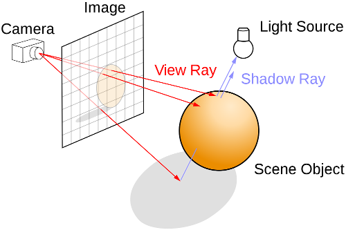
This process is illustrated by the image below (where the camera is at the eye position).
Test Cases
In tests.py, write test cases for cast_ray and
any auxiliary (helper) functions that you have written. You need not provide
test cases for cast_all_rays because this function prints
to the console. This will be tested in a different manner as discussed
below.
Casting Test
In casting_test.py, use cast_all_rays to create
an image using the following configuration. Be sure to print the P3
header to the screen before casting the rays. The width and height
are as specified and the maximum color value is 255.
Eye at <0.0, 0.0, -14.0>.
A sphere at <1.0, 1.0, 0.0> with radius 2.0.
A sphere at <0.5, 1.5, -3.0> with radius 0.5.
A viewport with minimum x of -10, maximum x of 10, minimum y of -7.5, maximum y of 7.5, width of 512, and height of 384.
When you run your program, redirect the output to a file named
image.ppm. This is done by typing the following at the
command prompt. (The first command, ulimit, which only needs
to be run once per terminal session, is used to limit the size
of the files generated. This will prevent a run-away program from
filling your disk quota.)
ulimit -f 12000
python casting_test.py > image.ppm
The image generated from this part should look like the following.
Though this is not the image we ultimately want, it is a useful image. The image indicates where intersections occurred, but it does not give much information beyond that. In fact, it is hard to tell that the scene contains two spheres. On to the next part.
Note: You can compare your generated image to the "expected" image using tools discussed at the bottom of this page.

A smaller image can be had by changing the viewport to the following
(this is only for debugging purposes; the casting_test.py
file that you submit must have the viewport set as originally specified).
Minimum x of 0.05859357, maximum x of 0.44921857, minimum y of 2.03125, maximum y of 2.421875, width of 20, and height of 20.

Part 2
To this point there is really nothing to make the spheres stand out. Let's add some color.
Data Definitions
Modify
data.pyto add a new class to represent aColorin RGB (red, green, blue) format. TheColor.__init__function should take argumentsr,g, andband initialize the corresponding attributes of the object. Be sure to define the__eq__function for this class.-
Modify
Sphere.__init__to takecolor(as its last argument) and to set the corresponding attribute of the object.
Functions
-
In
cast.py, update thecast_rayfunction to return the color of the sphere with the nearest intersection point (to the ray's origin), if there is an intersection, or a default color of white (1.0, 1.0, 1.0) if there is no intersection. Note: Do not make any assumptions about the order of the spheres in the array as relates to the nearness of the spheres.
Test Cases
Update your test cases in tests.py to reflect the changes to
these functions. Consider a test case for cast_ray that
verifies it will find the nearest sphere regardless of the order of
the spheres in the input array.
Casting Test
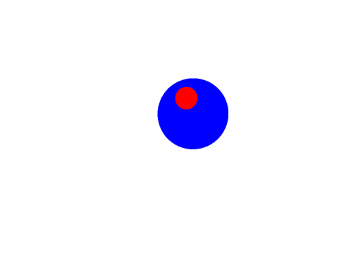
Update casting_test.py so that the smallest sphere is red and
the largest sphere is blue. The image generated from this part should look
like the following.
It is now apparent that there are two spheres in the scene (perhaps more, if some are hidden behind the others, but we know there are only two in this scene). Unfortunately, these spheres still look like circles. On to the next part.
And the smaller portion should look as follows.

Part 3
In order to give the scene some depth, and in so doing make the spheres actually look like spheres instead of circles, we need to add some notion of light. This will be done over these last three parts. Each part will add one component of the light model.
In order to implement the light you will need to add a finish to the spheres in the scene. The idea being that the finish "describes" how the object interacts with light (e.g., some objects are shiny while others are dull).
Data Definitions
Modify
data.pyto add a new class to represent aFinish. TheFinish.__init__function should, for now, take a single argumentambientand initialize the corresponding attribute of the object. This attribute represents the percentage of ambient light reflected by the finish. Be sure to define the__eq__function for this class.-
Modify
Sphere.__init__to takefinish(as its last argument) and to set the corresponding attribute of the object.
Functions
In
cast.py, updatecast_all_raysso that it expects aColoras its last argument. This argument is the ambient light color.In
cast.py, updatecast_rayso that it expects aColoras its last argument. This argument is the ambient light color.-
Update
Compute: Each component of the returned color will be computed by multiplying the corresponding component of the sphere's color by the ambient value of the sphere's finish and by the ambient light's color.cast_rayto modify the calculation of the color of the intersection point. If the ray does not intersect a sphere, then the returned color will remain the white default (1.0, 1.0, 1.0). If, however, the ray does intersect a sphere, then the returned color will now depend on the light model. At this point, the only contribution to the color will come from the reflected ambient light (think of the ambient light as a light that reaches everything).
Test Cases
Update your test cases in tests.py to test any newly created
functions and to reflect the changes to existing functions.
Casting Test
Update casting_test.py so that the scene's ambient light
is white (1.0, 1.0, 1.0; though you may experiment with other light
values, be sure to use this color for your submission). In addition,
the large sphere should have a finish with ambient value 0.2
while the small sphere should have a finish with ambient value
0.4.
The image generated from this part should look like the following.
This just looks like a darker version of the previous image but that is fine. The fact is, all that we really did in this step was set up the framework for the next steps and soften the color based on the ambient scale in each sphere's finish (if you increase the ambient scale, you can get the same image as in the previous step, but leave the values as directed for submission).

And the smaller portion should look as follows.

Part 4
For this step we will finally add some depth to the scene. This is accomplished by placing a point-light in the scene. Unlike the ambient lighting from the previous step, the point-light will emit light from a specified position.
Data Definitions
In
data.py, updateFinish.__init__by addingdiffuseas its last argument and by setting the corresponding attribute in the object. This attribute represents the percentage of diffuse light reflected by the finish. Be sure to update the__eq__function to reflect this change.-
In
data.py, add a new class to represent aLight. TheLight.__init__function must takept(aPointrepresenting the position of the light) andcolor(aColorrepresenting the color/intensity of the light) arguments and must initialize the corresponding attributes of the object. Be sure to define the__eq__function for this class.
Functions
In
cast.py, updatecast_all_raysso that it expects aLightas its last argument.In
cast.py,cast_rayso that it expects aLightas its last argument.-
Update
cast_rayto modify calculation of the color of the intersection point. In addition to the ambient component of the color, a sphere intersection will now also compute a diffuse component that contributes (additively, i.e., the result of the following calculation is added to the result of the prior calculation) to the resulting color.Consider the following options relating the intersection point on the sphere to the location of the point-light.
Note carefully that due to the imprecision of floating point values, using the computed intersection point in the following calculations can lead to unintended collisions with the sphere on which the point lies. To avoid these issues, these calculations will use a point just off of the sphere. This can be found by translating the intersection point along the sphere's normal (at the intersection point) by a small amount (use 0.01) (i.e., scale the normal by 0.01 to get a shorter vector and then translate the intersection point along this shorter vector). The following discussion refers to this new point as
pε.Compute
pεas just discussed.If the light is on the opposite side of the sphere from
pε, then it does not contribute to the color of this point. This can be determined by computing the dot product of the sphere's normal at the intersection point with a normalized vector frompεto the light's position. If the light is in the general direction of the sphere's normal (i.e., on this side of the sphere), then the dot product will be positive. If the dot product is non-positive (i.e., 0 or negative), then we will consider the light to be on the opposite side of the sphere's surface and, thus, it will not hit this point (so the diffuse light contribution is 0).Compute the sphere's normal at the intersection point. I will refer to this as
N. (This was already computed in order to computepεas described above).Compute a normalized vector from
pεto the light's position. I will refer to this asLdir.- Compute the dot product of
NandLdirand use this value to determine if the light is "visible" from pointpε.
If another sphere is on the path from
pεto the light's position, then the light is obscured and does not contribute to the color of this point. This can be determined by checking if a ray frompεin the direction ofLdir(computed above) collides with a sphere closer topεthan the light is.If the light is not obscured, then it will contribute to the point's color based on the diffuse value of the sphere's finish and the angle between the sphere's normal (at the intersection point) and the normalized vector pointing to the light.
More specifically, the light's diffuse contribution to the color of the point is (for each color component red, green, and blue) the product of a) the dot product between the sphere normal and the normalized light direction vector (i.e.,
N ˙ Ldir), b) the light's color component, c) the sphere's color component, and d) the diffuse scale of the sphere's finish.
Test Cases
Update your test cases in tests.py to test any newly created
functions and to reflect the changes to existing functions.
Casting Test
Update casting_test.py so that the point-light is located
at <-100.0, 100.0, -100.0> with color component (1.5, 1.5, 1.5).
In addition, the finish for each sphere should have diffuse value
0.4.
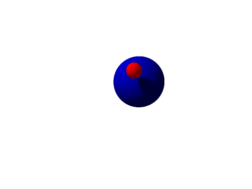
The image generated from this part should look like the following.
You can now see how light provides a depth to the objects in the scene giving an illusion of a third-dimension. You can also see evidence of the shadow effect caused when a sphere partially obscures the light from hitting another sphere.
And the smaller portion should look as follows.

Part 5
This last step adds some additional character to the image through greater distinctions between different finishes by computing a specular component to the light model.
Data Definitions
In
data.py, updateFinish.__init__to takespecularandroughnessas its last two arguments (in this order) and to set the corresponding attributes in the object. These attributes represent the percentage of specular light reflected by the finish and the modeled roughness of the finish (which affects the spread of the specular light across the object). Be sure to update the__eq__function to reflect this change.
Functions
In
cast.py, updatecast_rayso that it expects aPointas its last argument. This is the position of the eye in the scene.-
In
cast.py, updatecast_rayto modify the calculation of the color of the intersection point. In addition to the ambient and diffuse components of the color, a sphere intersection will now also compute a specular component that contributes (additively) to the resulting color.The specular contribution is computed as follows.
Compute the specular intensity by computing the vector that represents the direction in which the light is reflected and determining the degree to which that light is aimed toward the eye. You can do this as follows.
Create a normalized vector from
pεto the light's position (you already did this in the previous part). I will refer to this as the light direction,Ldir.Compute the dot product of the light direction and the sphere's normal at the point of intersection (you already did this in the previous part). I will refer to this as the light normal dot,
LdotN.Compute the reflection vector as
Ldir - (2 * LdotN) * N, whereNis the sphere's normal at the point of intersection.Compute a normalized vector from the eye position to
pε. I will refer to this as the view direction,Vdir.The specular intensity is the dot product of the reflection vector and
Vdir.
If the specular intensity is positive, then the contribution to the point's color is the product of the light's color component, the specular value of the sphere's finish, and the specular intensity raised to a power of [1 divided by the roughness value of the sphere's finish]. If the specular intensity is not positive, then it does not contribute to the point's color.
Test Cases
Update your test cases in tests.py to test any newly created
functions and to reflect the changes to existing functions.
Casting Test
Update casting_test.py so that the for each sphere has
specular value 0.5 and roughness value 0.05.
You can now see specular highlights from the light.

And the smaller portion should look as follows.

Handin
You must submit your solution on unix1.csc.calpoly.edu (or on unix2, unix3, or unix4) by 11:59pm on the due date.
The handin command will vary by section.
Those in Aaron Keen's sections will submit to the akeen user.
To submit Parts 1 and 2, at the prompt, type handin akeen 101hw4_1_2 data.py vector_math.py collisions.py cast.py casting_test.py tests.py utility.py
To submit your completed assignment, at the prompt, type handin akeen 101hw4 data.py vector_math.py collisions.py cast.py casting_test.py tests.py utility.py
Those in Julie Workman's sections will submit to the grader-ph user.
To submit Parts 1 and 2, at the prompt, type handin grader-ph 101hw4_1_2 data.py vector_math.py collisions.py cast.py casting_test.py tests.py utility.py
To submit your completed assignment, at the prompt, type handin grader-ph 101hw4 data.py vector_math.py collisions.py cast.py casting_test.py tests.py utility.py
Those in Paul Hatalsky's sections will submit to the grader-ph user.
To submit Parts 1 and 2, at the prompt, type handin grader-ph 101hw4_1_2 data.py vector_math.py collisions.py cast.py casting_test.py tests.py utility.py
To submit your completed assignment, at the prompt, type handin grader-ph 101hw4 data.py vector_math.py collisions.py cast.py casting_test.py tests.py utility.py
-
All of John Campbell's sections will use the same directory; submit to the jcampb25 user.
To submit Parts 1 and 2, at the prompt, type handin jcampb25 hw4_1_2 data.py vector_math.py collisions.py cast.py casting_test.py tests.py utility.py
To submit your completed assignment, at the prompt, type handin jcampb25 hw4 data.py vector_math.py collisions.py cast.py casting_test.py tests.py utility.py
Also, please handin any additional files, if any, that are required for your program to run.
Please note: the handin directory for parts 1 and 2 is different than the handin directory for the completed assignment.
Be sure to submit all files that are necessary to compile your program (including your files from the previous assignment(s)).
Note that you can resubmit your files as often as you'd like prior to the deadline. Each subsequent submission will replace files of the same name.
Grading
The grading breakdown for this assignment is as follows.
Clean Execution: 5% — Program runs without crashing (and the submitted source demonstrates a legitimate attempt at a solution).
Test Cases: 10% — Test cases are provided for each of the implemented functions. The number of test cases is appropriate for the complexity of the corresponding function (with a minimum of two test cases). The submitted test cases should be sufficient for the latest part completed (as submitted).
Style: 5% — Consistent formatting, reasonable variable names, and each line of code below maximum length (i.e., less than 80 characters).
Decomposition: 10% — Functional decomposition restricts each function to a single task. Duplicate functionality has been abstracted to a single function (i.e., duplicate code is removed).
Functionality: 70% — Required functionality has been implemented.
Sample Files and Comparing
Sample output images are given below (the earlier images shown in the browser are in a different format and are scaled down; do not compare against these). These are the images that should be generated by your system test for each part.
Image Diff Programs
You can compare your resulting image to those of the instructor solution with the following programs. Keep in mind, however, that there may be some legitimate minor differences due to the imprecision of floating point operations and the order in which your solution does computations compared to the order in the instructor solution.
There are two image diff programs available on the CSL machines.
They are ~akeen/public/bin/ppmdiff and
~akeen/public/bin/ppmdiff_analog. Each of these
programs takes two ppm P3 files as command-line arguments, reports the
differences between the files to the console, and generates a difference
image.
ppmdiff creates an image with a black pixel if the
corresponding pixel position differs between the two input files.
ppmdiff_analog creates an image with pixels colored by the
degree to which the corresponding pixel position differs between the
two input files. In short, the image from the first program highlights where
the differences are while the image from the second program gives a sense of
how "big" the differences are.