CSC 103 Lecture Notes Week 3

CSC 103 Lecture Notes Week 3
Trees, Part 1

Tree definitions
1. A tree is a multi-linked data structure consisting of nodes with pointers to two or more other nodes.
2. The connecting pointers between nodes are typically called tree edges.
3. A tree has a distinguished node called its root to which no other node points.
4. Recursively, a tree can be defined succinctly as empty, or a root node with edges to zero or more subtrees.
Tree views
1. There are a number of ways to depict trees in graphic form.
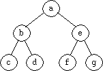
2. A standard textbook format shows nodes as labeled circles and edges as connecting lines; e.g.,
3. When we want to illustrate the implementation details of a tree, we'll draw them in the fashion we've used for linked lists, showing the actual pointers within the nodes, e.g.,
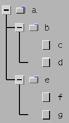
4. There are also a variety of ways that tree-like structures are shown in user- oriented formats; e.g.,
5. Lastly, when testing a program that implements tree data structures, it is convenient to view a tree in raw string format; e.g.,
```
a
  b
    c
    d
  e
    f
    g
```
  Here each vertical level of the tree is shown by indenting to the right two spaces, and (obviously) the edges are missing.
Terminology and facts
1. Tree terminology is a combination of botany and genealogy.
  1. The topmost node of the tree is the root.
  2. An upper node in the tree is the parent of the nodes immediately below it, and those lower nodes are the children.
  3. Nodes with a common parent are siblings.
  4. A node is the grandparent of nodes two levels below, etc.
  5. Nodes with no children at the bottom of the tree are leaf nodes.
  6. A path is a sequence of nodes connected by edges.
    1. The height of a node is the length of the longest path from the node to a leaf.
    2. The depth of a node is the length of the path from the root to that node
  7. This terminology is illustrated in Figure 1.
    
    Figure 1: Tree terminology.
2. The following are important tree facts.
  1. Every node except the root has exactly one parent.
  2. The root has no parent.
  3. There is a unique path from the root to any node.
Tree "arity".
1. In tree examples above, each node had two children; such trees are called binary.
2. In general, a tree node may have any number of children, from 0 to n; such trees are called n-ary.
3. Figure 2 is an example of an n-ary tree, depicting part of the CSC 103 file directory structure.
  
  Figure 2: Example n-ary tree.
Concrete data representations for tree nodes.
1. The most common data representation for a binary tree is an object with three fields: a data value, a left link and a right link:
2. This can be defined in a class definition such as the following:
```
class BinaryTreeNode {
    Object value;            // the value field
    BinaryTreeNode left;     // pointer to the left subtree
    BinaryTreeNode right;    // pointer to the right subtree
}
```
3. The data representation for an n-ary tree node code be done in a similar fashion, with a fixed data field for each subtree pointer.
  1. However, if there were a potentially large number of subtrees allowed this code be unnecessary wasteful of space.
  2. The typical solution is to used a linked list of subtree nodes, in a node of this form:
    
    where the children field points to a linked list of zero or more child subtrees and the next field points to the next child in a list of siblings.
4. This form of n-ary tree node can be defined in a class definition such as the following:
```
class NaryTreeNode {
    Object value;                 // the value field
    NaryTreeNode children;        // pointer to list of children
    NaryTreeNode next;            // pointer to next sibling
}
```
5. Figure 3 shows the concrete representation of the n-ary tree of Figure 2.
  
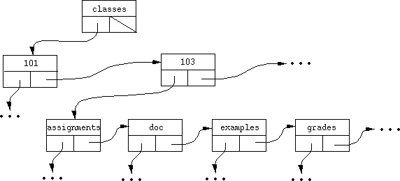
  Figure 3: Concrete view of an n-ary tree..
Binary tree example, focusing on tree traversal.
1. The attached program listing for BinaryTree.java illustrates the implementation of a basic binary tree.
2. The most fundamental operation on a binary tree is its traversal.
  1. Tree traversal is the process of visiting each node in the tree exactly once.
  2. Traversal of a two-dimensional tree structure requires a different approach than the traversal of a one-dimensional linked list we have looked at previously.
  3. In a linked list, we used a relatively simple for-loop to fully traverse the list.
  4. In a tree, a single one-dimensional for-loop won't do.
3. Here's a basic traversal algorithm for visiting all of the nodes in a binary tree:
  - If the root node of the tree is null, the traversal is done.
  - Otherwise, visit the root node.
  - Then recursively traverse the left subtree.
  - Then recursively traverse the right subtree.
4. This algorithm is called a preorder traversal, since it visits the root node first, then the left and right subtrees.
5. There are two other traversal algorithms called inorder and postorder that work in a similar fashion, but change the point at which the root node is visited.
  1. Inorder traversal:
    - Traverse the left subtree.
    - Visit the root node.
    - Traverse the right subtree.
  2. Postorder traversal:
    - Traverse the left subtree.
    - Traverse the right subtree.
    - Visit the root node.
6. The BinaryTree.findPreorder and BinaryTree.toString methods use a preorder traversal to do their work.
Binary search trees.
1. A particularly useful form of binary tree is called a binary search tree.
2. A binary search tree has the following property:
  For any subtree, including the full tree itself, all nodes to the left have a value less than the root and all nodes to the right have a value greater than the root.
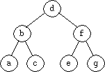
3. For example, the following tree contains the same nodes as in the figures on Page 1, but organized into a binary search tree:
4. The most appealing property of a binary search tree is that searching for a particular node can be performed using the following algorithm:
  - If the value we're searching for is at the root, success.
  - Otherwise, if the value is less than the root, search the left subtree.
  - Otherwise, search the right subtree.
5. If the tree is reasonably well balanced, this algorithm can operate in logarithmic time.
  1. This is the case because at each step in the search, half of the tree is eliminated from consideration.
  2. This is the same kind of logarithmic behavior we saw in the binary search of a linear list.
6. The attached listing for BinarySearchTree.java is a sample implementation.
Tree balancing.
1. The logarithm search behavior on a binary search tree only happens when the tree is reasonably well balanced.
  1. "Reasonably well balanced" means that O(N/2) of the nodes are in each half of the tree.
  2. The binary search tree property by itself does not guarantee a balanced tree.
  3. For example, Figure 4 shows degenerate "left heavy" and "right heavy" binary search trees.
    
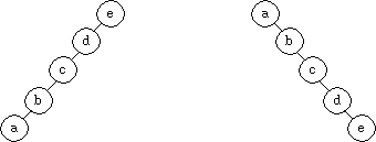
    Figure 4: Left-heavy and right-heavy binary search trees..
  4. In both of these trees, search time is O(N), not O(log N).
    1. This is because the "eliminate half the tree" step in the search algorithm ends up eliminating nothing
    2. So in the worst case, all N nodes of the tree must be searched to find the value at a leaf node.
2. The key to keeping a binary search tree useful is to maintain balance.
  1. This can be done by a global balancing algorithm, that takes any binary search tree and redistributes all of its nodes into a maximally well balanced tree.
  2. The problem with global balancing is that it is as expensive timewise as a complete sort.
  3. A more sensible approach is to maintain balance incrementally, not allowing the tree ever to get too far out of balance.
    1. Each time a node is inserted or removed from the tree, the tree balance is adjusted.
    2. The techniques to do this are illustrated by the AVL and red-black trees we will study next.
AVL trees.
1. An AVL (Adelson-Velskii and Landis) tree is a binary search tree with the following property:
  For any subtree, including the full tree itself, the height of the left and right subtrees can differ by at most 1.
2. This property meets the "reasonably well balanced" criterion to guarantee O(log N) searching performance.
3. Figure 5 shows two binary search trees; the one on the left is AVL, the one on the right is not.
  
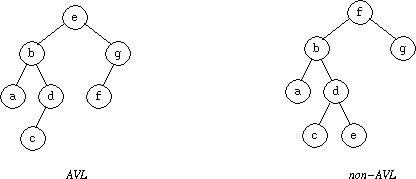
  Figure 5: AVL and non-AVL trees.
4. To maintain the AVL property, the tree must be rebalanced, if necessary, every time a node is inserted or deleted.
5. The key to the rebalancing is a rotation operation, that grabs an unbalanced tree by its proper root node and redistributes its out-of-balance children.
6. For example, suppose we have the following AVL tree to which we add a node with value c.
7. The steps to add the node then rotate the tree into balance are the following:
8. If we examine the possible ways that an AVL tree can go out of balance, there are four cases, which occur when a tree rooted at node has at least two levels:
  1. insertion into the left subtree of the left child of
  2. insertion into the right subtree of the left child of
  3. insertion into the left subtree of the right child of
  4. insertion into the right subtree of the right child of
9. Cases 1 and 4 can be handled by a single rotation; cases 2 and 3 require two rotations.
10. We will now examine the examples in Sections 4.4.1 and 4.4.2 of the book that illustrate the different cases.