

This project is based off of Jos Stam's 2003 GDC paper for real-time fluid dynamics. I have always been fascinated with fluid dynamics and simulating it through programming. My implementation is certainly not optimal but illustrates my understanding from an introduction graphics course and a quick overview of fluid dynammics.
Fluid dynamics is the science of liquids and gases in motion, it ranges from air to water to more! This project will illustrate a fluid simulation in two dimensions. One could imagine water on a flat table with a very small border enclosing the liquid, when moving their finger through the water they would be applying forces to the liquid. The program is simulating that real world interaction, hence the term fluid simulation!
To us this simulation may seem pretty real and that is truly all we want when it comes to video games and visual effects. There is a big difference between the simulations of fluids in video games and movies versus those to test airplanes and automobiles. The latter need to be extremely accurate, while the former just needs to look visually appealing, enough so to sell an audience. The solver layed out by Jos Stam is catered toward the visual appealing and is not intended to perfectly model fluids.
Turns out for a two dimensional simulation the most important pieces of data we need are density and velocity. So how does this help?
The simulation implements an N x N grid (defaults to N = 128). Each cell in the grid contains two pieces of information, it's current density and velocity. A cell's density represents how much of some matter is present. An its velocity represents the forces present in that current cell, this directs the flow of density and provides movement! In the case of this simulation the density will be displayed by color! More on this later.
For the technical, the grid is represented by parallel arrays, a density array and a vector array. For efficiency purposes the arrays are single dimensional and indexed as though they were two dimensional. An extra layer of cells surrounds the N x N grid to help with boundary conditions.
We start with an initial velocity and density, in our case no velocity and no density are present in the grid when we first run the program. As time passes the grid is updated with the information present in the grid itself, this information comes from the user! By right clicking the mouse the user adds density to a cell, by left clicking and dragging the user begins to add forces (which are added to the cells velocity vector) in the direction of the mouse!
There are three main steps to moving densities:
Adding forces allows us to move the density around, we want movement and flow! As more forces become present at each cell the densities in said cells begins to move out of their current cell and into the next, to simulate this each cell kind of looks around to the other cells and see what will direction those cells are. This lets each cell decide where to pull in densities from (we will expand on this in just a second). Next we need to realize that as densities begin to move around the grid they enter some cells and leave others and speed up or slow down, this is diffusion! Diffusion applies to both densities and velocities, eventually the fluid should slow down and dissipate accross the grid. Now I mentioned "pulling" in density from neighboring cells. In our advection step we have two sets of data the previous "snapshot" of the grid's density at the last time step and the new grid's density values. Now at each cell we trace backwards through the velocity field. One could think of it as pulling in density at each cell instead of pushing out density at each cell. We are literally just one step ahead :). And just like that we have movement, this is done over and over to give us a great fluid simulation!
Evolving the cell's velocities over time is very similar to densities but another step is added. A projection step, this allows us to force the velocities to be mass conserving giving us more realistic fluids. For more information on the velocity step I encourage you to check out Jos Stam's paper linked at the bottom of the page!
The first video is a lower resolution (32 x 32 grid) to illustrate the vector and mesh views. The second video is a higher resolution (128 x 128 grid) to illustrate a nicer looking simulation!
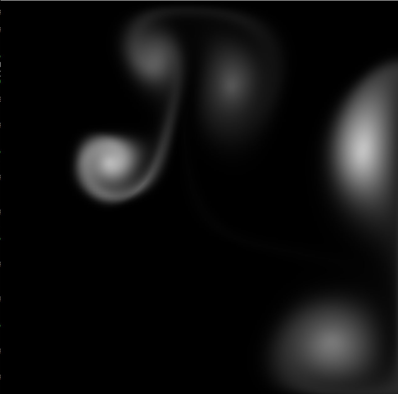
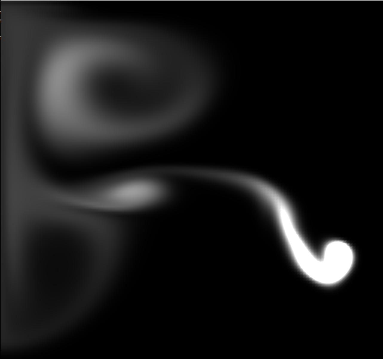
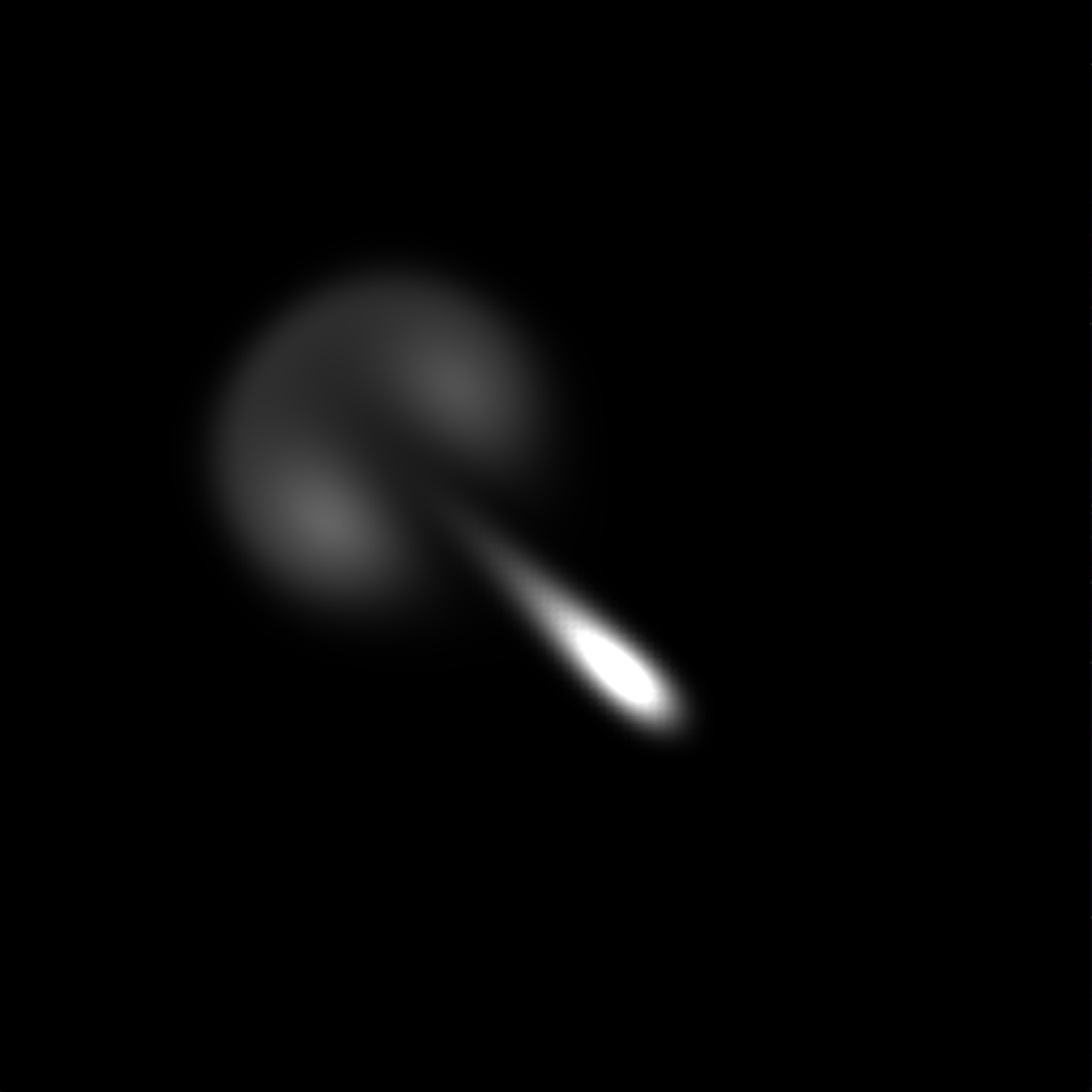
The "smoke" mode is a grayscale representation of densities throughout the grid. It looks a lot like smoke and is a good example that looks like something we would find in the real world.
The density heat map mode gives us better insight on the amount of density per cell. The scale is blue, green, yellow, red. Red being the most dense and blue the least dense.
The vector mode shows the vector field that the density is following. The first screenshot has 128 x 128 cells and the second one has 32 x 32 cells, the third shows the heat map view as well. The smaller grid is to better illustrate the vectors themselves.
The cell mode is to illustrate the representation of data on the GPU. Each cell is composed of two triangles, each triangle has three vertices, each vertex has an (x, y) component. For a 128 x 128 grid we have 16,384 cells, that's 32,768 triangles, and 98,304 vertices... which means 196,608 xy values. Our arrays get huge. This can be optimized using indexing to avoid sending the same vertex multiple times, but one can see that this can get difficult to scale, especially when we want three dimensional simulations.
Fluid simulations are pretty straight forward but the math definitely gets complicated sometimes. Storing the data and representing it properly is challenging and certainly comes at a cost. I learned a lot about OpenGLs buffered objects and saw a lot of room for optimization that could have been done if allotted more time. In the future I would love to extend this to three dimensions and optimize the solver and move it to the GPU instead of ramping up my CPU on this. Also utilizing textures would eliminate a lot of the overhead of passing a huge array of color values per vertex.
Please check out Jos Stam's paper! He does an amazing job explaining real-time fluid dynamics for video games and there is a ton of other works he has done on this topic.
If needed feel free to contact me at joncatanio at gmail. Or check out my personal website for other methods.