Simple Inverse Kinematics

Kolton Yager
CPE-471 Spring 2017

Introduction to IK

Inverse kinematics is a technology commonly used in both computer graphics and robotics to enable intuitive manipulation of systems of moving parts. In particular, for computer graphics it's used in animation and games to make the posing of arms, legs, and similar limbs easy and/or procedural. The fundamental idea behind inverse kinematics, is to find the inverse of the forward kinematic equation. The forward kinematic equation simply being the equation determining the location of some object. In the typical case this is the end of some kind of limb, i.e. a hand. In scenarios such as this the system is characterized by a chain of rigid segments or, in the terminology of CG character rigging, bones which hierarchically rotate and where the endpoint is the tip of the last bone. These types of bone chains are fundamental in character rigging for posing different limbs.

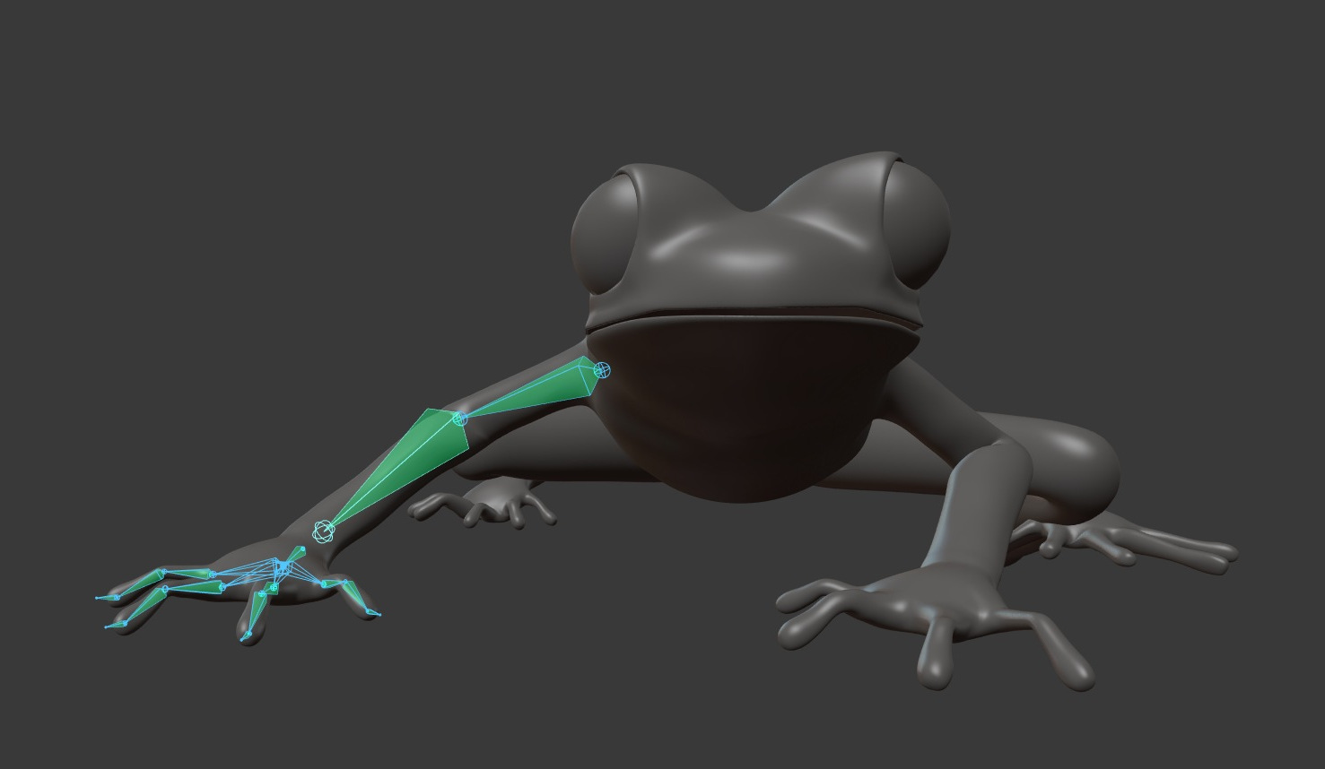
However, animating a limb such as this by rotating each bone into position every time so that the endpoint lands in the correct position is tedious and unintuitive. Instead most animators want to be able to move the endpoint itself, and have the rest of the chain follow suit. For this reason, we attempt to find the inverse kinematic equation. If successful, this allows such an endpoint to be moved freely, with the bones posing automatically to follow.

Setting Up the Foundation

My goal for this project was to implement a simple inverse kinematics scheme with the tools we've gained from CPE 471. The structure to solve for being a chain of bones with an endpoint controlled freely. Before any inverse kinematics could be done I had to set up a framework for objects and their relationships to other objects. I decided to largely re-work all of the base code that we've used in the class thus far, throwing out the reliability on global variables and creating new Object classes that have their own inherent affine transformation and which can be freely parented to one another. This parenting allows for easier hierarchical modeling as during the draw call for any object, transformations are applied recursively from child to parent until the base geometry is reached at which point actual drawing calls are made. This functionality is then extended to create the Skeleton, bones, and IKcontroller subclasses which are used for the actual IK. The skeleton mostly acts as a container for the set of bones, and the IKcontroller acts as a special added on child of a Skeleton object which influences bone position and stores the details of the active IK.

Prior to being controlled in a non hierarchical fashion, the bones need to be set up to work hierarchically. Initially I attempted to do this with the same affine transformation stack used by parented objects. However, it ended up being easier to instead store bones like individual unit length segments with a location and direction, then resolve their transformation independently from any other transformation matrices. Eventually I was able to get the bones to work in general and maintain constrained movement relative to one another as demonstrated below where each bone has it's own simple animation.

Implementing Jacobian IK

There are a variety of approaches and algorithms that can be used for inverse kinematics in computer graphics. However one of the most direct methods is built around the Jacobian. The Jacobian refers to the Jacobian matrix, which is a special matrix formed from partial derivatives of a function with vector output and its various inputs. In the context of inverse kinematics, the Jacobian matrix represents a matrix representation of how changes in the orientation of bones in the chain influence change in the endpoint. In the abstract we can say subsequently write the following equation which essentially states that the change in location of the endpoint is equal to the Jacobian multiplied by the change in the angles in the bones.

$J∆e = J·∆\theta$

As a result, if we want to find find how much the angle of each bone changes based on how much the endpoint has changed instead, we can do some algebra which will tell us that we instead want

$J^{-1}·∆e = ∆\theta$

Where we multiply the inverse Jacobian matrix by the change in the endpoints location. This is not a simple task however. As you may know, finding the inverse of a matrix is not an easy or necessarily possible task. First, if a matrix is not square, which the Jacobian is very often not, the standard definition of an inverse matrix no longer applies. As a result, alternate methods of finding a pseudo-inverse that will essentially work as we desire. The simplest way to do so is simply by using the transpose of the Jacobian. This is a very crude estimation of the inverse, and as will be discussed later is more prone to error. Instead, it is better to use the Moore-Penrose Pseudo-Inverse which is defined for all matrices square or not. The formula for which is below

Where A* is the transpose of the matrix in question. There is however a problem here in that this formula involves another inverse, which is also not always possible. While multiplying the matrix by its transpose does create a square matrix, in certain situations it is still not invertible. In order to find a guarenteed solution, I instead use Singular Value Decomposition which is a method that after being used on the Jacobian, will allow for an easy computation of the inverse.

Now that the inverse Jacobian is calculated it can be used to solve the inverse kinematics for the chain. One of the inherent problems with inverse kinematics is that the solution to our inverse kinematic equation is not unique, there are technically infinitely many solutions to the equation. As a result the best we can ever do is to approximate the posing/motion we want. Furthermore, the calculation of the solution using the Jacobian inverse is also just an approximation, so it must be used iteratively to find valid values and it should be kept in mind that no solution is perfect. In my implementation, this iterative solution is done every time the endpoint's position is updated. First, I measure the difference between the endpoints old and new location. Next, this distance is subdivided into smaller movements if the movement is large. For each subdivision (even if just one) the an IK function is run which calculates the Jacobian inverse and uses it to rotate the bones in the chain by a very small amount is run many times. Each time the solver is run the bones are only rotated a fraction of the amount the solution suggests so that subsequent iterations will be more accurate. With this, I have created a basic IK solver which you can see applied below. First using the Jacobian Transpose to solve, then using the Singular Value Decomposition Pseudo inverse

Jacobian Transpose Solution

Jacobian Inverse Solution

As you can see, the transpose solution has a somewhat more error prone solution compared to the inverse. They both have points of failure, which I believe is a result of the lack of restrictions and some simplifying assumptions made about the rotational axis of the bones. However, it does clearly show the foundational effectiveness of the Jacobian as a method for IK solving, and with more refinement could be implemented as an effective and flexible IK solver.

Sources

Aristidou, A., & Lasenby, J. (n.d.). Inverse Kinematics: a review of existing techniques and introduction of a new fast iterative solver (pp. 12-17, Tech. No. CUED/F-INFENG/TR-632). CUED.

Buss, S. R. (n.d.). Introduction to Inverse Kinematics with Jacobian Transpose, Pseudoinverse and Damped Least Squares methods (Tech.). University of California San Diego.