Graphics Technologies Utilized
- • Blinn-Phong Shading Model
- • Game Camera
- • Auto-screengrab for later video render
- • Texturing
- Skybox
- Various models
- • Jos Stam Fluids
Program Controls
- • WASD + Mouse for camera movement
- • X to add smoke coming out of the volcano
- • P/O,L/K,M/N for adding velocity to the smoke. Each pair of keys alters the velocity in one dimension of the cube.
- • C to clear the simulation of all velocity and smoke.
Fluid Solver Explained - Simulation
The simulation of the fluid takes place in two distinct parts: the velocity solver and the density solver.
The velocity solver is the more complicated of the two. It simulates a velocity vector field which is a combination of the previous frame's vector field and any added velocity sources. Then, in order to let future computations be easier and make the fluid more realistic, it alters the vector field to make it mass conserving. Next, the velocity diffuses around the simulated environment, in my case a box, causing a more stable vector field to emerge if no more velocity sources are added. The velocities of the vector field are then applied to the fluids in your environment, moving them accordingly.
The density solver is a bit simpler than the velocity solver, as it basically uses a subset of the velocity solver code. Here, after the fluid has ran through the velocity solver, any new fluid sources are added to your simulated environment. Then, all of the fluid diffuses. This means that regions of high density become less dense, sharing their mass with the regions around them. Similarly, regions of low density accept mass, absorbing it from their surrounding regions.
Fluid Solver Explained - Rendering
The main question I hoped to answer when approaching this project was if a reasonably-realistic 3d smoke could be rendered in real time. At least with Jos Stam's algorithm, this is completely impossible.
On a laptop, the highest resolution I was able to run the simulation at with a decent frame rate was 12x12x12. On a desktop, this number got up to around 16x16x16. Unless you're playing MineCraft, these resolutions aren't going to cut it.
However, if you're willing to wait a long time for rendering, some extremely realistic smoke can be achieved. Examples of this can be found in the section below.
Although I did answer the question of if this could be ran in real time, I didn't really scratch the surface of how my render could be improved. My method was essentially creating a threshold value for the amount of smoke necessary in a given cube for it to be rendered, and then rendering the whole cube if that value was met. Possible extensions to this project could include rendering the cube a different color depending on the density/velocity value present there, adding transparency based on cube density, or implementing some multithreading to decrease frame render time.
Example Renders
|
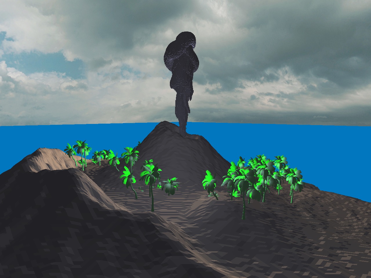
Still shot at 24FPS. Simulation Resolution: 75x75x75 Total frames rendered: 500 Time to render: ~1 hour Time per frame: 7.2 seconds |
|
|---|---|
|
Rotating shot at 24FPS. Simulation Resolution: 75x75x75 Total frames rendered: 500 Time to render: ~1 hour Time per frame: 7.2 seconds |
|
|
Rotating shot at 24FPS. Simulation Resolution: 125x125x125 Total frames rendered: 300 Time to render: 4 hours Time per frame: 48 seconds | |
|
Rotating shot at 24FPS. Simulation Resolution: 175x175x175 Total frames rendered: 300 Time to render: 12 hours Time per frame: 144 seconds |
Resources
- Real-Time Fluid Dynamics for Games, Jos Stam
- Jos Stam’s Fluid Simulations in 3D, Softology's Blog
- Tropical palm, killst4r
- 3D RedRock, Toafaloaf
- Mount Vesuvius, Conor O'Kane
- Easter island Moai Free 3D model, y4juzn
- Jos Stam Browser Implementation, BlainMaguire
- Output Image to file, RigidBody
- FFMPEG
- All scenes rendered on an ASUS Chromebook Flip running GalliumOS