This program was created as the final project for CSC 471 at California Polytechnic State University. The program described below is a 2D real-time fluid simulation based on the 2003 GDC paper by Jos Stam. It was implemented in modern openGL version 3.x, glew, and glfw for a windowing program.
In this section, I will cover the basics of a real-time fluid simulation. I really recommend checking out Jos Stam's paper as it covers it extremely well.
Fluid simulations are a really really fast way of representing fluids in games and graphics. Some simulations require precise estimation of real life behavior, however, if all we really care about is visual appearance we are allowed to cut some corners. Since we aren't simulating water erosion against a bridge or other critical system, we can use a less computationally intense and more stable solution. This allows us to represent fluids in a simple, cheap, but convincing way!
When it comes down to it, all it takes to represent a fluid is a velocity, and the density of the fluid. In the context of this program, the density of the fluid is really just how much "stuff" there is at a given point. The velocity can be represented as a direction, negative or positive, and a magnitude, or how strong that force is. So at any given point we should have some kind of density, and that density should have a magnitude and a direction telling it where to go.
So at this point, you're probably wondering: "Well how do I turn this into code?" which means it's time to go over some data structures.
What we really want to do is make a bounded area where our fluid can bounce around in. The best way to do that is represent the fluid in a square grid such as 64x64 "cells." Where the cell is a location that has some amount of density and a velocity. The best way to do this is to have two parallel arrays, one that represents density, and the other that represents velocity at any point.
Great question! There are three major steps to answering the question of: "Where is that density, and where is it going?" First the density should have some sort of initial position with no forces acting on it. It just kind of exists. Then the next logical thing to do is add forces! We want to make it move! Wait...There are other densities as well...So where do those go? Well each cell exchanges a little bit of itself with the cells surrounding it and it also receives some density from its neighbors. This is known as diffusion and it happens with both densities and velocities. The amount of density that is exchanged or received is dependent on the velocities at each of those cells, and similarly for the diffusion of the velocity. The third and final step is to move that density! We now know how much density we've received from neighboring cells, and what our velocity is so let's move in that direction! From here we just repeat all three parts of the simulation by adding new forces, diffusing, and moving our densities!
Unfortunately, it isn't that simple. There are a few more complex concepts to deal with such as advection, and projection, but that is the basics! If you are thirsty for more details or the nitty gritty details of the Navier-Stokes equations, then check out Jos Stam's paper!
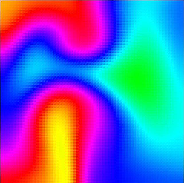
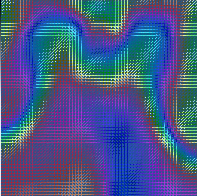
Above are some basic examples of what a filled grid with the color shader enabled. The different colors are different amount of densities, and the really cool shapes that the fluid is making is because of the velocity field! Since our velocity diffuses as well as our density, even if we only add velocity at one position the density will continue to move in different directions from the source until the velocity diffuses enough to become zero.
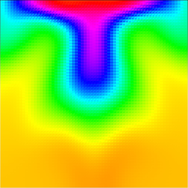
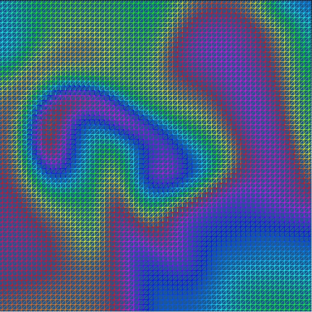
Well that's pretty cool, but what would it look like if we wanted to represent something other than a lava lamp? Here we can see a smoke like simulation that could pass as the smoke coming off of a fired gun or smoke filling a bottle. The only thing that changed between the smoke and the colorered pictures was the shader. That means we can represent many different types of fluids that behave the same way by just changing the color!
Remember how we said we were going to represent fluids by parallel arrays for density and velocity? Well each index into that array represents a cell in our grid that needs to be representing by 6 vertices. We need 6 vertices since this is modern openGL and GL_QUADS is deprecated! So each grid cell is actually made up of two triangles that have their own interpolated color.
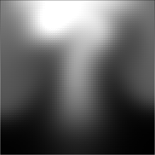
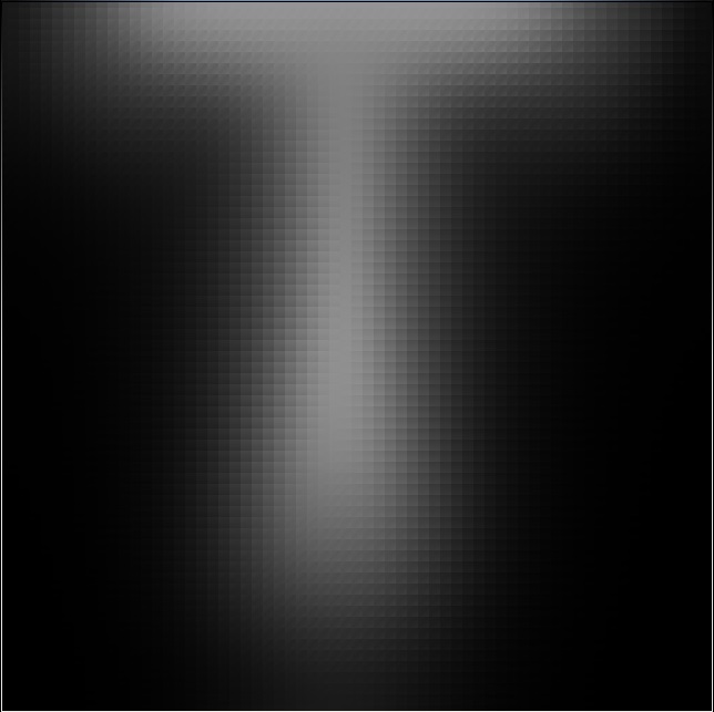
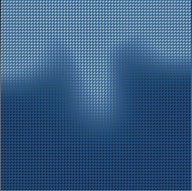
Good thing we have a mesh view! Below you can see four examples of the fluid simulation with all of the triangles shown that represent our grid!

Well from here there are a couple of things that we could do. We could find a better way to represent our data. Currently we have a 64x64 grid with 6 triangles per cell! That's 24576 vertices... This significantly limits our ability to scale up this simulation. Similarly we can change this to a 3D simulation by doing all of our steps, but instead of a 2D grid we have a 3D grid.
The two most important things I learned from this project was how to properly deal with VAO's and VBO's to store my vertex data, and how much leeway we have in non-critical graphical simulations.
Contact me at njlemay at gmail dot com