Austin Quick — CPE 471 — 03/23/2017
One of the most challenging domains in computer graphics is the pursuit of photorealism. In theory, to achieve perfect realism, one must first simulate the universe. This is not currently a possibility. Thus, in practice, all known solutions are approximations. The smaller the approximation, the greater the complexity.
One can imagine a spectrum containing some of the commonly used “realistic” rendering strategies, ranging from most to least approximated…
Phong Shading → Ray Tracing → Path Tracing
Phong shading yields very convincing results for ambient, diffuse, and specular lighting from specific kinds of light sources. It is extremely useful in that it does this very quickly. The drawback is that for more complex lighting factors (shadows, reflections, ambient occlusion, etc.), additional mechanisms must be implemented, each a large approximation in its own way, and each reducing overall performance.
Ray tracing requires a considerable leap in computational cost, but trivializes shadows, reflections, and refractions, amongst other things.
Path tracing again requires a considerable leap in computational cost, but tackles what’s known as global illumination. In theory, given enough time and resources, it will yield the most realistic result.
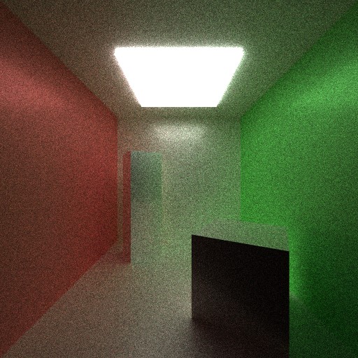
Path tracing, although extremely computationally expensive, is surprisingly intuitive. Essentially, individual rays of light are traced backwards from the camera through the scene. If a ray intersects an object in the scene, the material properties of the object determine if and how the ray is reflected or refracted. Once the ray either escapes the scene or intersects a light, it is terminated.
Overall Program Flow
The program works iteratively, one frame per sample. Each iteration traces a random ray through each pixel and adds the resulting color to a running per-pixel total. This has been parallelized on the CPU to a user specified number of threads, where each thread corresponds to a pixel. If, for instance, the program was to be run with two threads, the first thread would process all even pixels, and the second all odd. After an iteration has been completed, the data is uploaded to the GPU and rendered as a static quad.
Once all samples have been calculated, the final colors are averaged, and the result output as an image.
Ray Generation
The camera’s location, orientation, and field of view, as well as the aspect ratio of the screen provide information enough to define a frustum. This frustum differs from a typical perspective frustum in that it lacks a near or far plane. For each pixel of each iteration, a unit length ray is calculated that originates at the camera location and passes through a random point of the pixel’s square.
Ray Tracing
Each ray is intersected with the scene, and the nearest collision is processed. If there is no collision, the ray is terminated. If the collision is with an emissive entity, the light color is multiplied by the ray’s factor, added to the ray’s destination pixel, and the ray is terminated. At this point, there is potential for a child ray. If the depth of the child ray were to exceed the user specified maximum, the ray is terminated. If the factor of the child ray were to be less than the user specified minimum, the ray is terminated. Otherwise, a child ray is generated and replaces the current ray.
Child Ray Generation
A child will probabilistically fall into one of four categories: super-diffuse, super-specular, sub-diffuse, and sub-specular. Super child rays are those which reflect off the surface. Sub child rays are those which refract through the surface. Diffuse child rays are those whose angle of incidence is independent on the parent’s. Specular child rays are those whose angle of incidence is dependent on the parent’s.
Whether the child will be super or sub is determined by the material’s transparency. A transparency of 0.0 will result in exclusively super rays. A transparency of 1.0 will depend entirely on Fresnel’s equations whether or not the child ray reflects or refracts. A transparency in-between affects the probability linearly.
Whether the child will be a diffuse or specular is determined by the material’s specularity. A specularity of 0.0 will result in exclusively diffuse rays. A specularity of 1.0 will result in entirely specular rays. A specularity in-between affects the probability linearly. Additionally, the specularity determines the cone angle of the child ray if it is specular, linearly interpolated between ??/2 at specularity 0.0 and 0.0 at specularity 1.0.
Diffuse Rays
Diffuse rays are generated randomly on the unit hemisphere defined by the surface normal.
Specular Rays
Specular rays are first generated as a random vector in (not on) the unit sphere. This vector is then scaled by the radius of the tangent sphere of the cone defined by the angle determined by the specularity of the material. The angle is the angle between the cone axis and the cone perimeter. The radius of the tangent sphere is equal to the sin of the cone angle. The vector is then translated by the cone axis normal and then normalized. The end result is a random distribution of unit vectors within a cone around the reflection vector, with a higher probability toward the center.
Collision Detection
In a scene with potentially millions of triangles, determining through which any arbitrary ray passes first has the potential to be extraordinarily costly. To speed things up, the scene space is split into a hierarchical tree structure known as a KD-tree. The idea of the KD-tree is to recursively split an axis aligned bounding box along its longest axis such to minimize s1n1 + s2n2 , where s is the surface area of each sub-box and n is the number of elements in each sub-box. The KD-tree is created once at the start of the program, and traversed for each ray-scene intersection.
Absorbance
Rays that pass through translucent materials are subject to loss in intensity in accordance with their absorbance as dictated by Beer’s law.
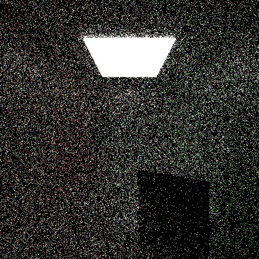
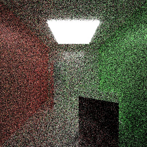
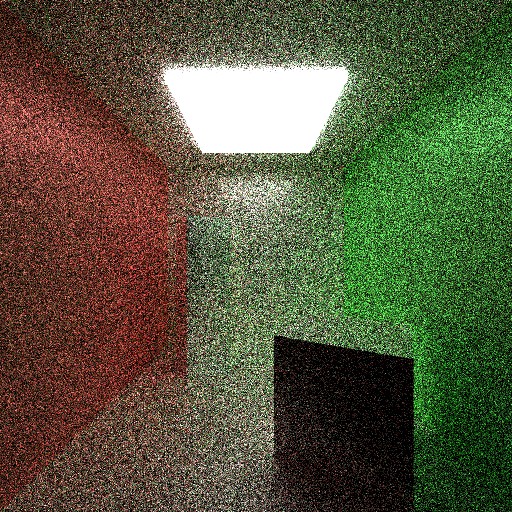
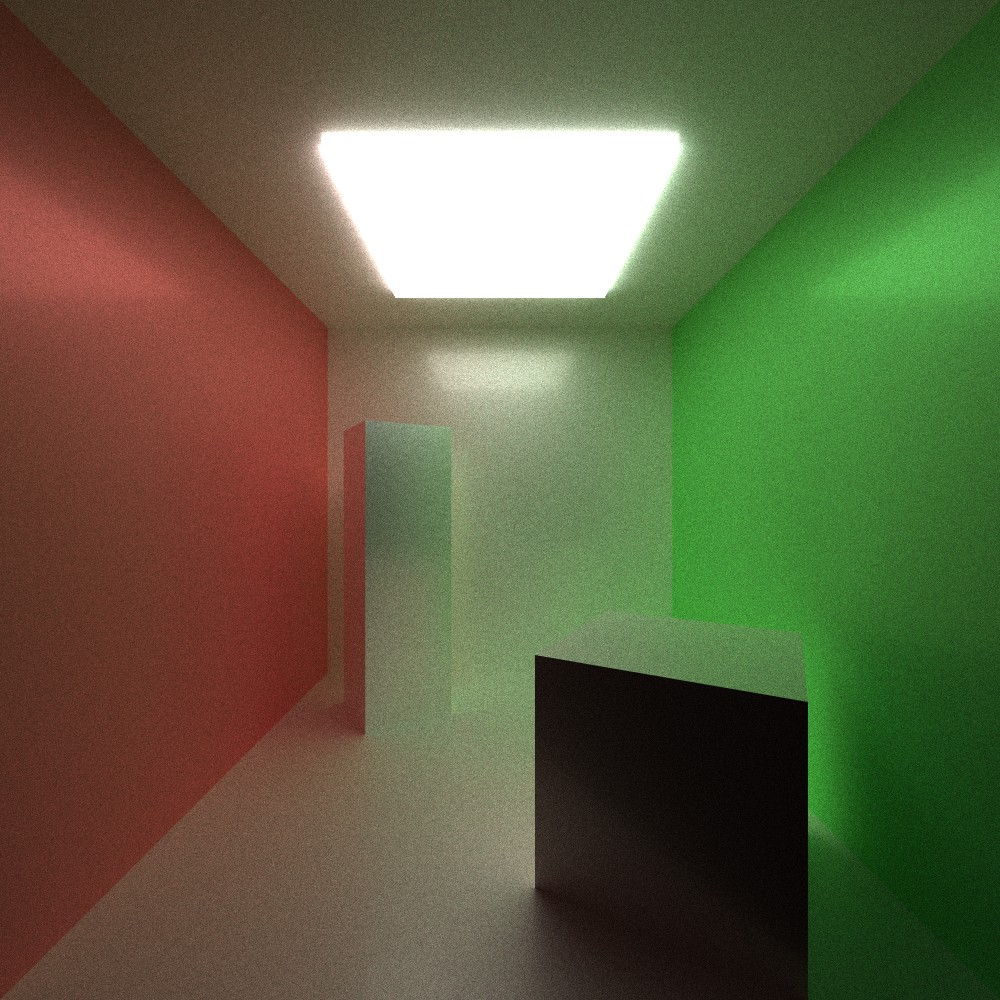
An unfortunate, if iconic, artifact of path tracing is graininess. Graininess is exponentially proportional to the number of samples (number of rays cast) per pixel. In order to halve the graininess, the number of samples must double. The below series of images demonstrates this property.
1 Sample:
2 Samples:
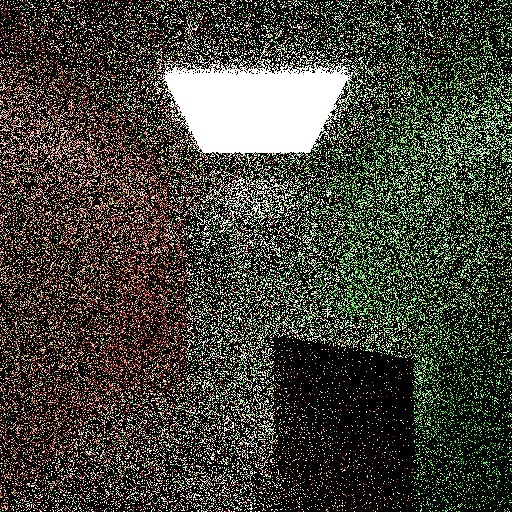
4 Samples:
8 Samples:

16 Samples:
32 Samples:

64 Samples:

128 Samples:

256 Samples:
512 Samples:

1024 Samples:

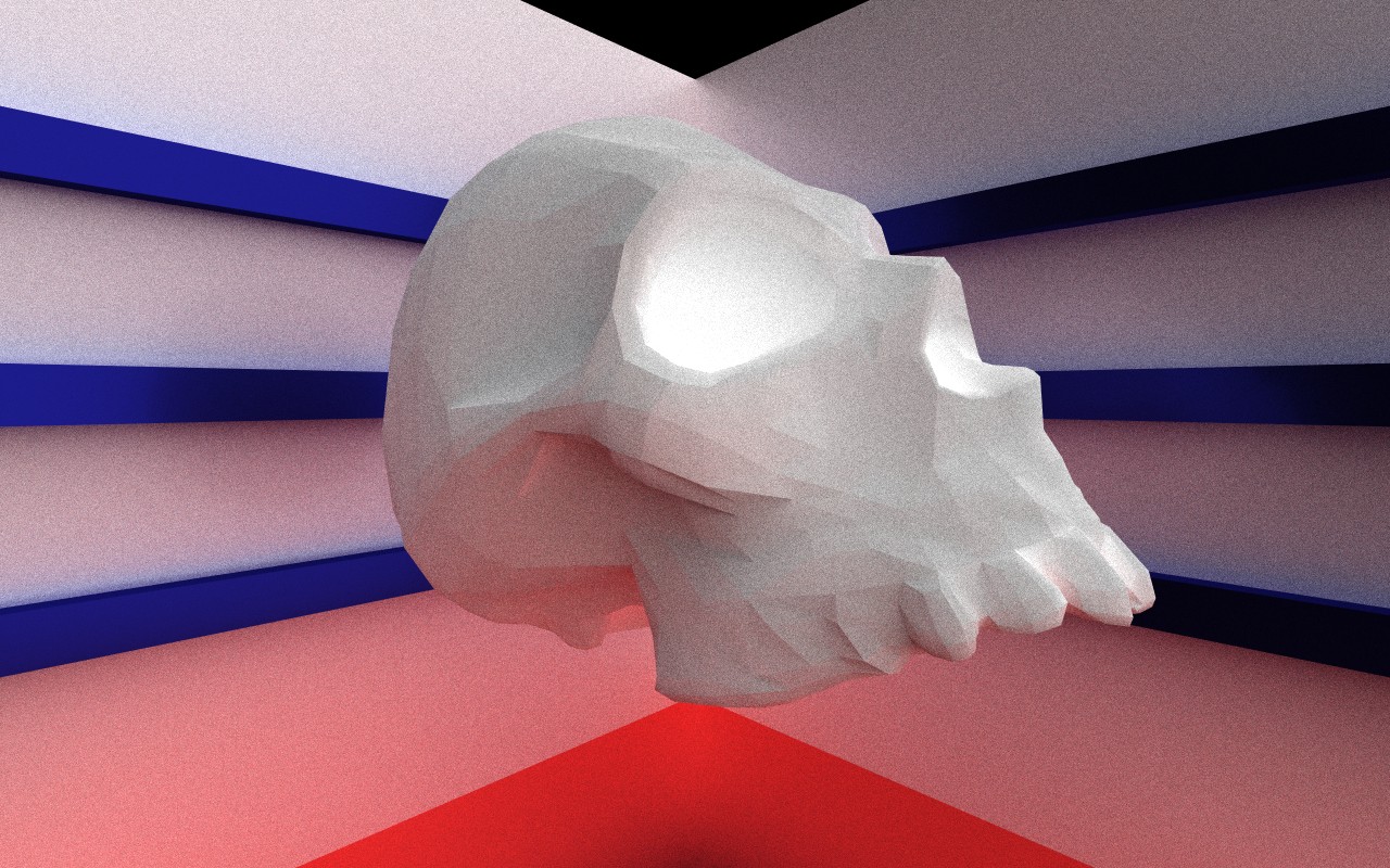
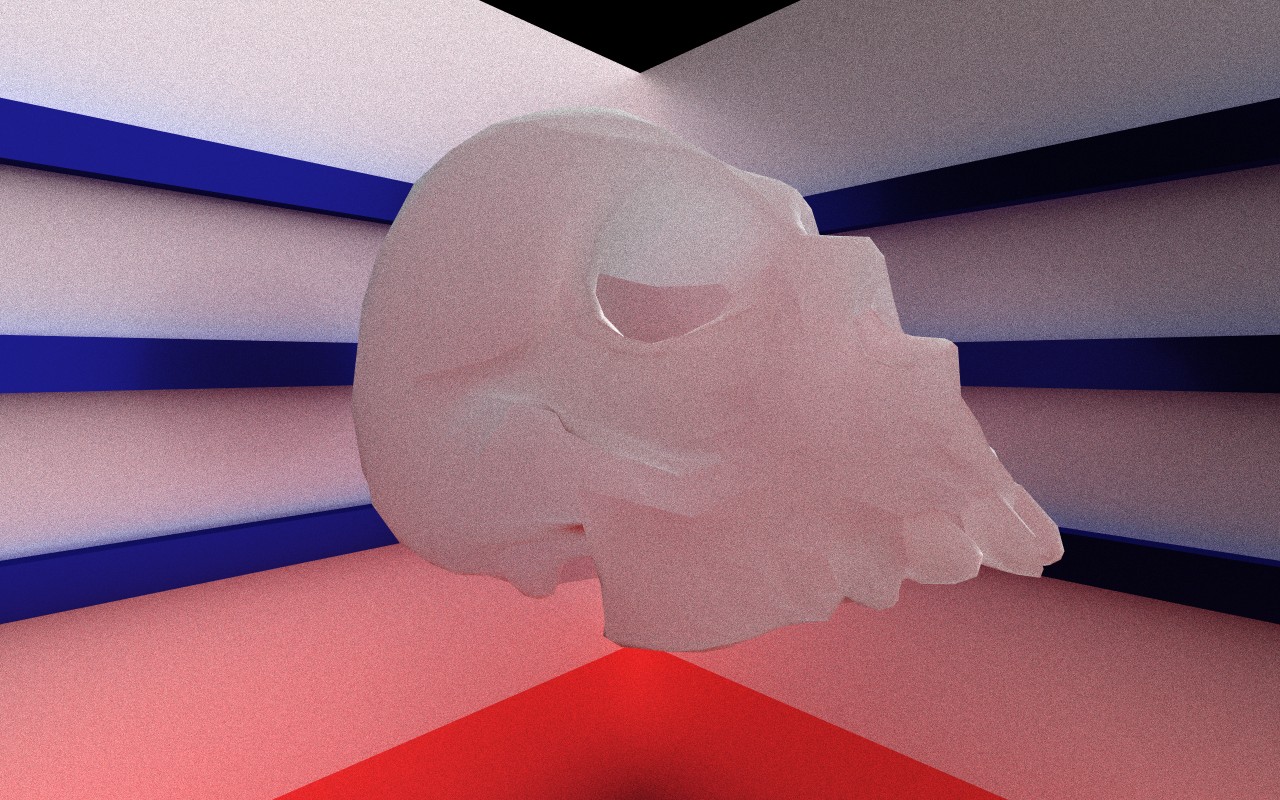
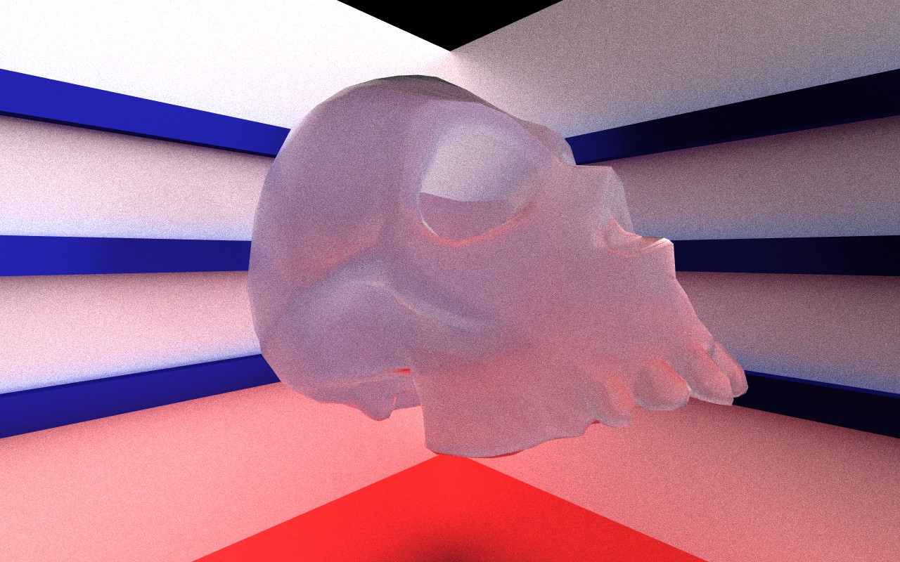
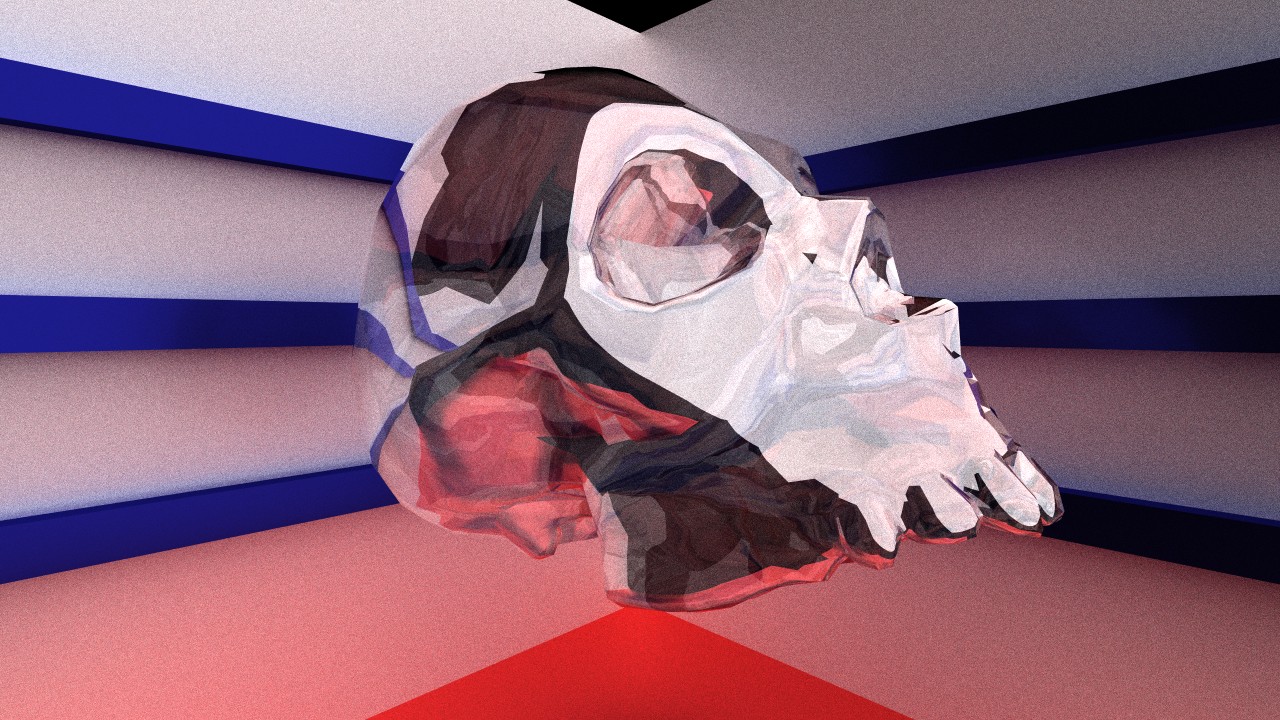
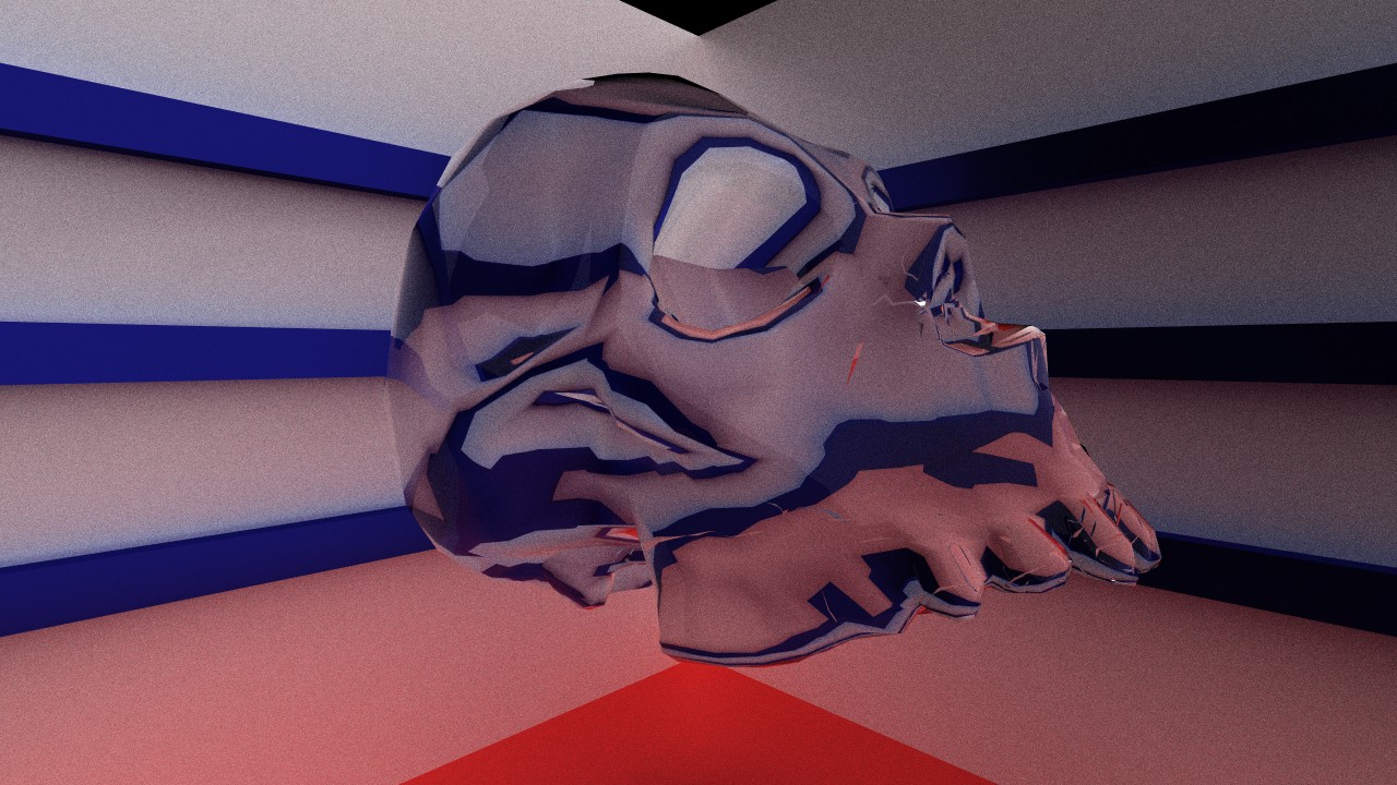
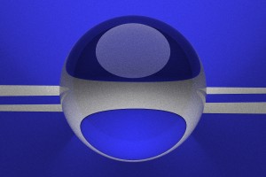
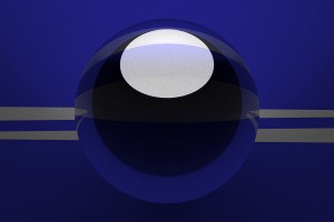
A demonstration of the effects of specularity and transparency.
Specularity 0.0, Transparency 0.0 (pure diffuse)
Specularity 0.0, Transparency 1.0 (pure internal diffuse)
Specularity 0.75, Transparency 1.0 (blurry glass)
Specularity 1.0, Transparency 0.5 (mirror glass)
Specularity 1.0, Transparency 1.0 (glass)
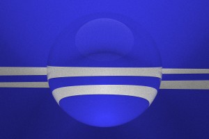
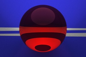
A demonstration of the effect of index of refraction.
Index 1.2 (less than ice)
Index 1.5 (typical glass)
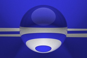
Index 2.0 (greater than sapphire)
Index 10.0 (no known materials)
Colored glass
Full Size (1000 samples)
Just for fun
Photon mapping to allow for higher fidelity at lower samples and enables caustics and narrow-access lighting in a sane amount of time.
GPU implementation to drastically increase performance.
Ingo Wald's Thesis on real-time path tracing
Reflections and Refractions by Bram De Greve