

For this final project I decided to accelerate our quarter long ray tracer program through parallelization. Because images produced by the renderer are naturally represented by a matrix, this process can easily be parallelized through multi-threading using #pragma directives in openmp. However, because I had remote access to a supercomputer I decided to distribute the program over multiple processors. The key distinction between distributed computing and multi-threading is that when distributing a program, we run the same process across multiple nodes rather than having multiple threads run in one process. Consequently, one node cannot not have access to another node's program space and must use a message passing interface to communicate.
The ray tracer has 2 main steps: parsing the scene then casting the rays to determine the color of each pixel. Because parsing is a process that doesn't contribute much complexity to the program, I decided to have every single node parse the input file rather than having only the master parse. This allowed me to avoid dealing with the overhead of sending the objects to each of the n-1 nodes. Then, the actual raytracing was distributed by assigning each node a specific set of rows to render. After the nodes complete their assignment, they send its results back to the master for the final write of the image. Rows were assigned in a non-consecutive fashion so that when given a scene in which geometries are concentrated in one area, each node's load is relatively balanced.
The non-trivial aspect of this problem lies in the inability to send nicely formatted C++ data types and objects across nodes. This is every single node must parse the input file on its own. All messages are just blocks of memory bytes which must be formatted by the sender and receiver. This is done using a tool called MPI which stands for Message Passing Interface. MPI's API allows me to send these chunks of memory to and from each node in a distributed system. By specifying the data type and size of the chunks of memory I want to send, I can use MPI to flatten the arrays and send them to the master to be written to the final output image. Each node including the master does this and after, the master will sequentially fill its pixel matrix and write the values to the output file.
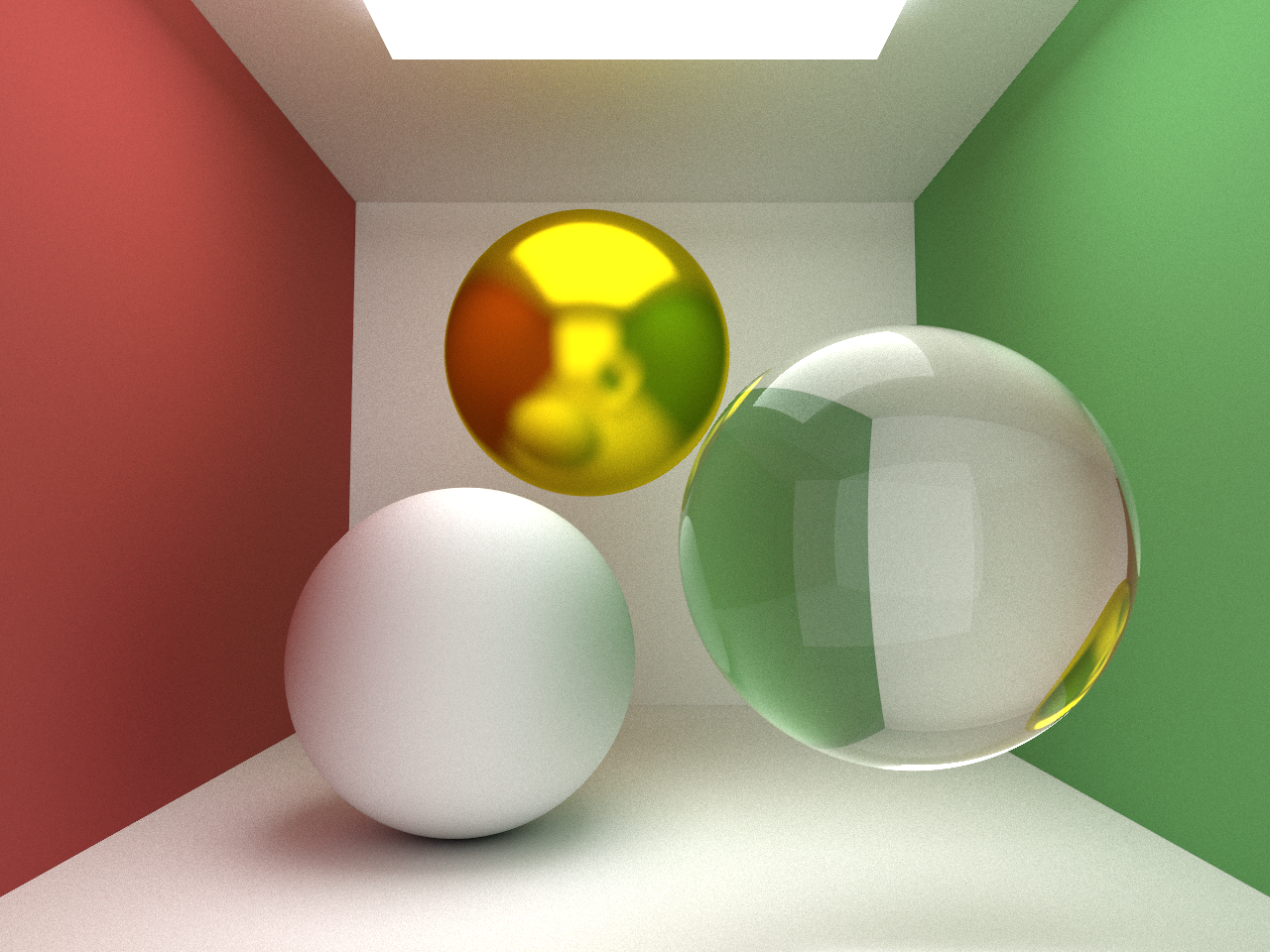
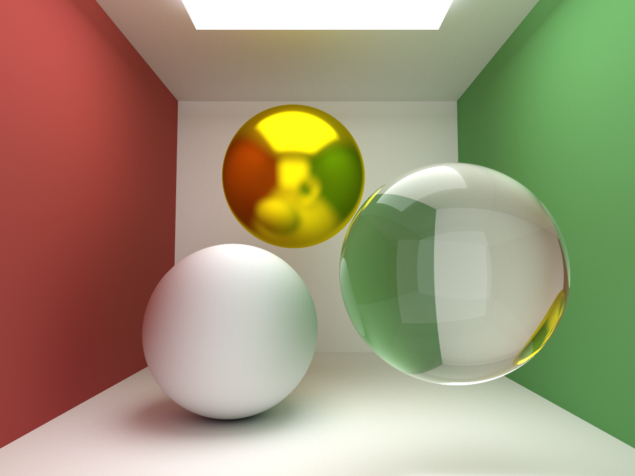
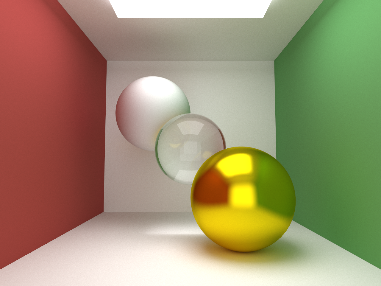
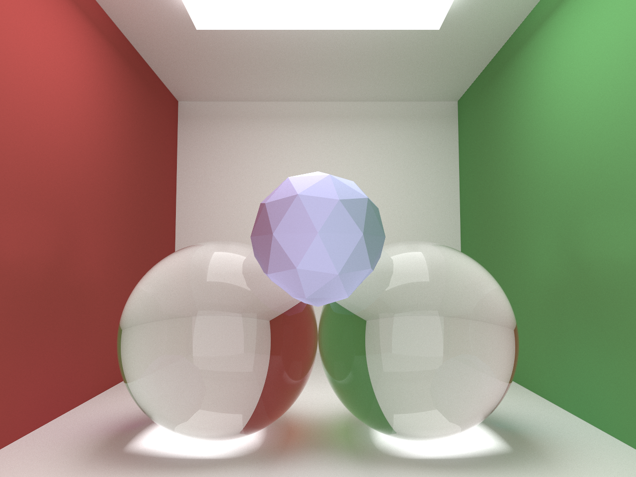
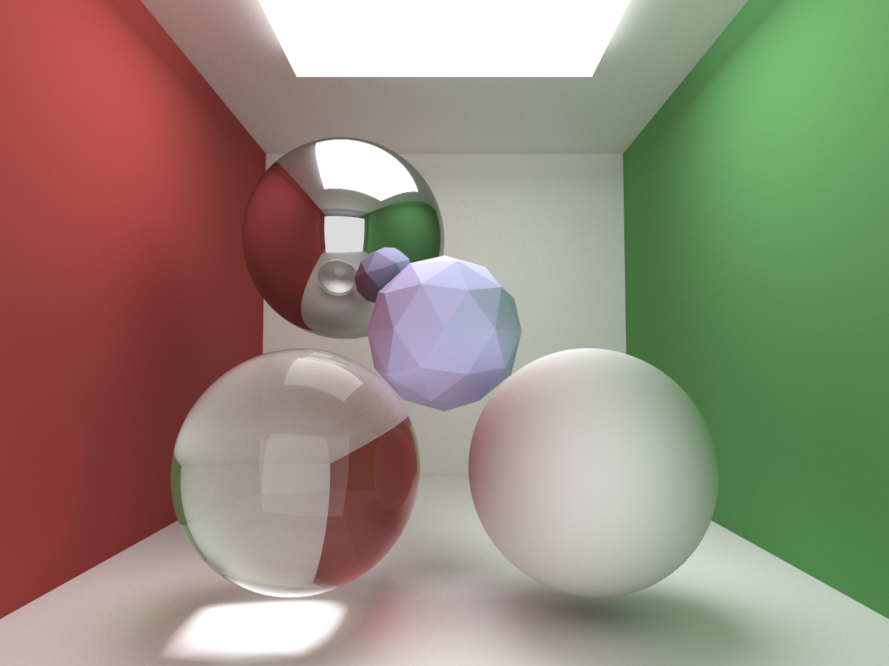
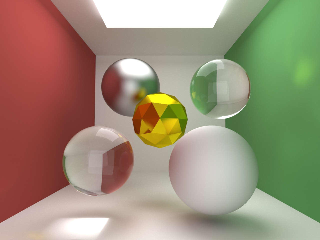
Scenes of the Cornell box containing objects of various shapes and materials were rendered. Timings were taken for execution on a single node on the PSC Bridges supercomputer as well as for execution using 48 nodes for comparison.
The results of this acceleration were somewhat unexpected but unsurprising. After timing the execution of the renderer using sample sizes of 100, 400 and 800 on a single node and then on 48 nodes on the supercomputer, there was an average speed up of 14.95 rather than the expected 48. However, after assessing the state of the ray tracer, I realized that these results should not come as a complete surprise. I predict that one of the reasons for this is due to the lack of a bounding volume hierarchy (BVH). Although each node is responsible for a specific portion of the image, we must still test for an intersection with every single object which exists in the scene. In addition, rays casted into the Cornell box are guaranteed to hit some object and are highly likely to bounce around multiple times before exiting the recursion. Another possible reason for such small speedup could be due to the overhead of using MPI and waiting for all n-1 (47 in this case) to report back to the master node before creating the final output matrix (n^2).
This speedup still allowed for a much larger sampling of rays leading to significant noise reduction and more beautiful images in less time. Overall I am happy with the results of this acceleration. However, more work can be done to further accelerate the renderer such as implementing a BVH, using a different sampling method such as importance sampling and implementing further parallelization through openmp within each node.