Edge Detection, Normal Mapping, and Depth of Field

Project Description

The goal of this project is to Add 3 new features to the CSC 473 ray tracer. They are edge detection, normal mapping, and depth of field. For edge detection, object outlines, self-occluding edges, and object intersection lines are shaded as hard black edges. For normal mapping, the program reads in a new type of parameter in the povray format and applies the specified normal map file to the sphere (like texture mapping, this only works on spheres). For depth of field, a focal distance and lens aperture are defined in code and the produced image produces a focal effect, blurring objects not at its focal distance. Because two of the 3 features listed require multiple extra sample rays per ray cast, a minor obj hit detection upgrade was created as well.

Gif example of particle flow

Command Line Arguments

a.out <width> <height> <input_filename> <output_filename> <shading_model> <numRays_perPixel> <recursionDepth> <optional_obj>

Edge Detection

To achieve edge detection each kind of edge must be accounted for. First, to detect literal edges of the object view we cast a disc of sample rays around and parallel to the original base ray. If any sample ray does not hit the object, we can return the base ray as an edge. If all rays hit the same object, we then check at what distances they each hit. If any distance is significantly different than the others, we can return the base ray as an edge. Finally, for object intersection we test all sample rays to determine if they hit any other object before hitting the base object, and if so we return the base ray as an edge. The last type of edge which this code does not correctly find is crease edges. a possible solution is to check if any hit distances is more than some amounts of standard deviation away from the mean of the rest of the hit distances.

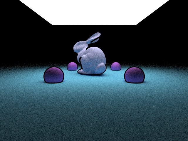A bunny surrounded by four spheres, all 3 edge types are shown: outline edges, object intersections, and self-occluding edges.

Normal Mapping

While normal mapping is similar to texture mapping, an important difference is the need to transform the normals recieved from the normal map image into object tangent space. This is due to the typical nature of a 2-D image being pointed in a single direction (at the "camera"). To achieve this, a transform matrix is produced called a TBN (Tangent, Bitangent, Normal) matrix, and is represented on the sphere shown below.

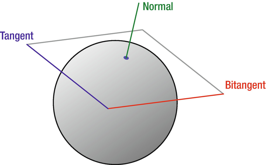Tangent space represented on the surface of a sphere

This matrix is generated after detecting a spherical hit. The t variable can be thought of as the "up" vector of the surface, b can be thought of as the "right" vector, and n is the already known normal. After applying this matrix to the current normal, a new normal is produced based on the normal map texture.

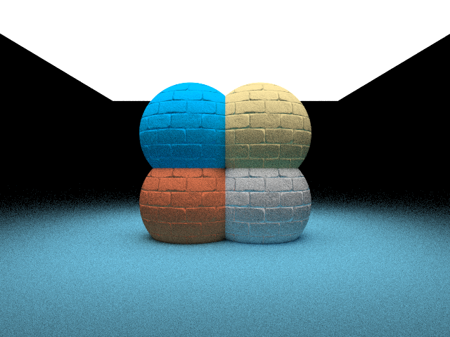Rendered using a brick normal map on each sphere

Depth of Field

Depth of field is achieved by more realistically simulating a pinhole camera, at least moreso than we already are. Currently, we generate a number of random rays for every pixel on a supposed "image space" and cast them into the scene to recieve lighting data. Depth of field requires that rays act more like a pinhole camera, all passing through a single point before spreading out, as seen below.

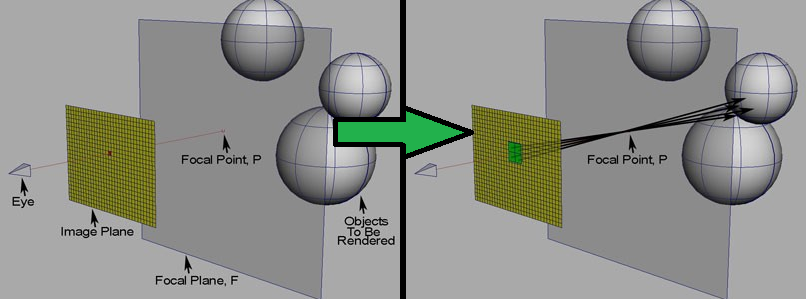Visualization of depth of field ray tracing

To accomplish this, for every ray we send out into the scene, we generate a number of sample rays around it, all pointing to the same spot at a certain distance along the original ray. This distance is the focal distance, and the radius at which these samples are generated is the aperture radius. These rays are then cast into the scene as well, and instead of taking the original ray's lighting data, we average out the sample rays' data. After doing this for every ray cast, we achieve a simulated depth of field. Below are some examples.

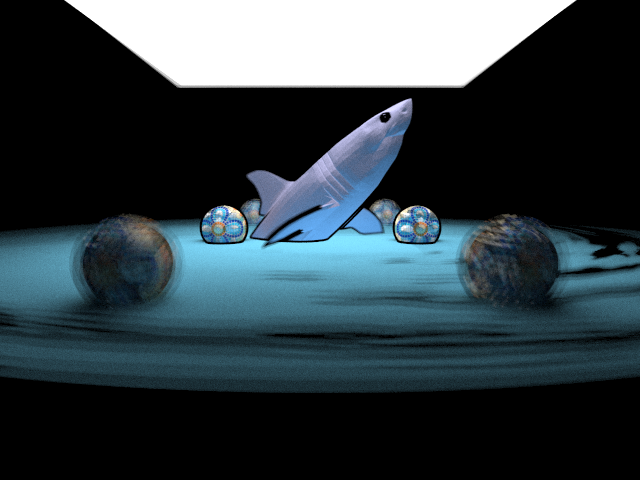
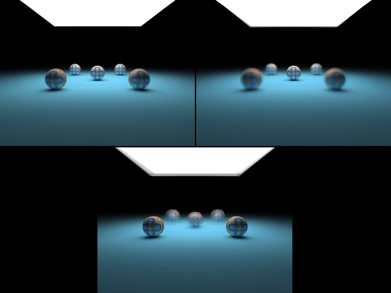Three examples using depth of field rendering. Top Left: focal dist = 10, r = 0.1. Top Right: focal dist = 10, r = 0.25. Bottom: focal dist = 7, r = 0.25.

Faster Obj Hit Detection

Due to the number of additional sample rays that must be cast by these new features, a slight speedup was added to the obj hit detection system. While not as fast as a BvH tree, this still shows significant improvements in speed over the old system of checking every triangle if a ray hits the object's bounding box. Some sample times measured include an image taking 3m20s to render down to 1m40s, as well as another going from 6m45s down to 3m25s. This can be conceptually simplified as thinking of putting each triangle in a bounding sphere as big as the largest triangle in the mesh.

In full, we track of some maximum distance for the ray to perform a small sphere intersection test within the bounding box. If all a triangle's points are not within this distance, we can skip that triangle and move on to the next. This maximum distance is calculated during obj loading, and is set to half of the longest edge distance on the triangle with the largest area. This was determined because if a ray hits anywhere within a triangle, the farthest distance it can be from the closest point is half that longest edge distance.

Optimizations may be made to this algorithm and logic, as this is highly dependent on triangles of a mesh being somewhat regular between one another; for example, if a mesh has a single triangle whose edge spans the entire length of the mesh.