Aligning sets of 3D data point is an important step in reconstructing real-world geometry from many discrete 3D samples. While iterative optimization techniques can be sensitive to noise and susceptible to locally optimum solutions, stochastic optimization techniques such as RANSAC can find semi-optimal alignments even when substantial noise is present in the input. We apply GPU parallelism to this process with CUDA, producing reasonable solutions in a timely manner.

The problem of acquiring 3D representations of real world geometry is an important and thoroughly studied problem in computer graphics and computer vision. There are many different digital sensors available for sampling the structure of 3D scene, and all (being digital sensors) produce one or more discrete 3D data points per sample. Commonly, each data point contains a position and sometimes a color, and the sets of 3D data points are referred to as a “point cloud”. Frequently many such point cloud samples of a single scene are taken from different locations and viewing angles, and it is desirable to be able to use all of this information together to resolve the structure of the scene being sampled. However, since the sensor always measures the 3D data points relative to itself, each of these point clouds is expressed in the space of the sensor at the time the sample was taken, which can change relative to the worldspace between samples. Thus it becomes necessary to determine the relationship between these sampling spaces so that all of the point clouds can be unified and operated on together as a single cloud. This is fundamentally a problem of fitting a mathematical model (a rigid transform relating the two sampling spaces) to a data set (two point clouds in different sampling spaces) based on an objective function measuring the quality of the fit.

RANdom SAmpling Consensus (RANSAC) is a general technique for fitting mathematical models to data points which operates by taking many random minimum samples from the data set (where each sample is just large enough to compute a single model), evaluating the objective function on each of these models, and then keeping the model which fits the data set most closely. Traditionally this is done iteratively, terminating when the probability of finding a better sample falls below a certain margin, but parallel implementations which evaluate a fixed number of samples and keep the best one have also been investigated.

In this paper we discuss the application of RANSAC to find rigid transformations relating the sampling spaces of two point clouds, and then demonstrate a parallel implementation of RANSAC optimized for this application which leverages NVIDIA’s CUDA API to achieve efficient parallel evaluation of the objective function specific to this application.

Often a set of samples of 3D data from a single viewpoint is insufficient to reconstruct an entire model or scene at the desired level of detail (as many types 3D geometries cannot be imaged completely from a single viewpoint). This requires that multiple sets of 3D samples be merged into a unified space for processing, which requires resolving the relationship between the two sampling spaces. While this relationship can be input by hand or estimated with a transformation sensor such as a GPS receiver or 3-axis accelerometer, most of the time this comes down to optimizing some measure of total distance between the points in the cloud. Some methods for achieving this include Simultaneous Location and Mapping (SLAM) [2] and Iterative Closest Points (ICP) [3], which can be used in conjunction with one another or other algorithms to achieve highly accurate and robust point cloud composition [1].

Iterative optimisation techniques, such as ICP, are susceptible to finding local minima as solutions, and thus requires a good initial guess of model parameters [1], which often is not present. RANSAC is a general model that offers a solution to this problem by taking a ‘shotgun’ approach to optimizing a model to fit a data set. By testing a random sampling of possible solutions, RANSAC is not vulnerable to cornering itself into a locally optimal solution that might not be the best global solution.

In general the use of RANSAC to optimize point cloud alignment involves the following steps:
 1) Select a minimum sample set from cloud
 2) Use each minimum sample set to compute the transformation which maps one sample set onto the other
 3) score the estimate transform by summing the square of the distances between the closest points in the sets
 4) repeat 1-3 until the probability of finding a better transform drops below a preset probability threshold

The first description of the RANSAC is in a 1980 paper[4]. It outlines a general approach to solving the problem of fitting a model to experimental data. One example specifically given in the paper is matching a set of 3D coordinates their possible locations in a 2D image, which is similar to goal of this project. One problem with other approaches (such as “least squares”) that RANSAC was meant to solve was the issue of the “poisoned point”, a gross error in data collection that can throw off the whole estimation.

More recent papers have covered the applications of RANSAC in respect to scene reconstruction from multiple sets of 3D information [5, 6]. In this application, there are many advantages over the iteratively based approach
 1) RANSAC often produces better results, even in noiseless cases
 2) RANSAC does not require a good initial estimate of the transform between the two data sets
 3) RANSAC can be used with data sets that do not have as many local features

Optimizations, such as pre emptive culling of unsatisfactory hypotheses were implemented to help cut down on the time spent processing this wide-reaching and largely unguided algorithm. One method outlined in [6], calculates the scores for each hypothesis in a “breadth first” manner, calculating a small portion of the score and comparing it to the rest of the scores to see if it is still worth pursuing.

A combination of optimization techniques outlined in [7] results in image pairs being matched at above real-time speeds (55Hz+). These optimizations were tailored to the use-case and included improving model verification, the initial hypothesis generation, and preemptively discarding underperforming hypotheses.

In our implementation the RANSAC function takes as input two point clouds, A and B, and tries to find the transformation matrix M which maps cloud B into the space of cloud A, such that M*B “fits” with A as best as possible. This notion of “fitting” is somewhat poorly defined for point clouds, and one common approach for quantifying it is as follows

For each point p_b in B apply M to p_b and find the point p_a in A which is closest to M*p_b. If the distance between p_a and p_b is below some predefined inlier threshold then p_a is an inlier for model M. The model with the most inliers is considered optimal.

Because measuring the success in this manner requires searching one (potentially very large) point cloud for a closest match to every point in a different (also potentially very large) point cloud (where each closest neighbor search is completely independent of all others), the evaluation of the fit is simple to parallelize. Additionally, RANSAC functions by randomly sampling and evaluating the fit of a large number of potential hypotheses independently of one another, which offers another point at which the computation can be easily parallelized.

Our primary contribution is a parallel implementation of a RANSAC optimized specifically for the purpose of aligning sets of 3D data points (point clouds) which parallelizes both the scoring of different hypothesis transformations and the nearest neighbor search for each point per hypothesis. Because the process of scoring of many hypotheses involves applying many different transforms to the same large set of points (B) and checking these many transformed points (M*B) against the same large, un-transformed point cloud (A) , CUDA’s shared memory model allows a cooperating block of threads to evaluate many transformations with a very high compute to global memory access (CGMA) ratio.

When developing our implementation, we started off with a classical iterative structure so that we could test the component functions of the point cloud alignment (such as transform computation from minimum sample sets) without having to worry about subtle errors being introduced during parallelization (of which there were several). Once the iterative code worked correctly we parallelized our implementation using as much shared code as possible. This allows us to compare the runtime of two very similar implementations of the same algorithm, where the only difference between the two is the parallelization of the hypothesis evaluation.

Our test platform an ASUS Zenbook Prime UX32VD laptop with a 1.9GHz Intel Core i7-3517U, 6GB DDR3 RAM, and an NVIDIA GeForce GT 620M GPU with 96 CUDA cores. In the following tests we are matching point clouds of about 1670 points each. The runtimes below do not include the file IO, point cloud creation, or feature matching. They are runtimes for two functions which take a pair of pointclouds, a set of matched feature points, and the number of random samples requested and return the best random estimate within that sample size. The two functions use rand in the same way (they generate random samples with the same function) and srand(0) is called before each run, so the transforms returned by the serial and parallel versions are always the same. Following are graphs of measured performance, varying the number of random samples between 0 and 1024, incrementing the number of samples by 8 each test.

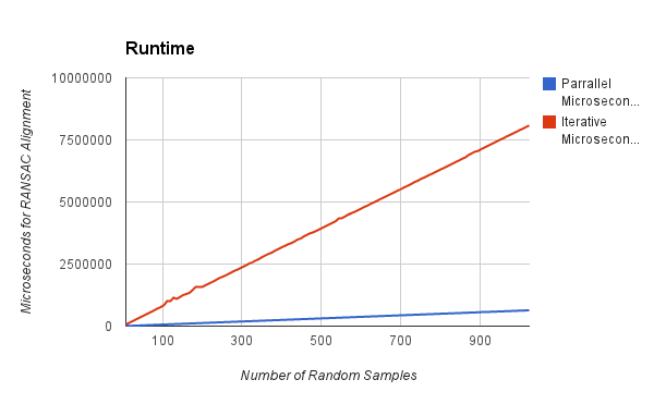
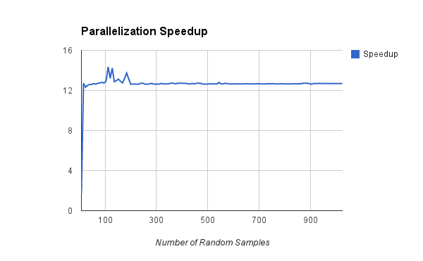
There is very little to note here. Both runtimes show essentially perfectly linear growth with respect to the sample size and the speedup is almost perfectly constant across the entire test sequence. Because each hypothesis has a block dedicated to evaluating its fit, we expect that the speedup would scale up with increased GPU SM’s.

One thing I found particularly interesting is the blurb of noise in the iterative data between 100 and 150 samples. This noise results from the burst of CPU activity when I closed all the other programs I was running and left the laptop to finish the test suite. When I discovered the noise I re-ran the test suite with nothing else running from the start, and the results were substantially smoother over that region, but I kept the original data here because I think it illustrates an interesting point. As you can see from the graphs above, scheduling hiccups on the CPU increase the speedup of GPU acceleration because the GPU is not subjected to these same scheduling conflicts. This illustrates a rarely discussed allure of GPU programming: that modern personal computers are hybrids of serial and parallel hardware and, at least right now, far fewer programs are using the GPU for general purpose computation. So, while the CPU side of an application is fighting hundreds of other applications for CPU scheduling time, the GPU side can be happily humming away on a monstrous parallel coprocessor with little or no resource contention (and also not be taking up valuable processor time which other applications need to function). Of course GPGPU is very young, and this could all change very quickly, but it remains an interesting note.

When developing our implementation, we started off with a classical iterative structure so that we could test the component functions of the point cloud alignment (such as transform computation from minimum sample sets) without having to worry about subtle errors being introduced during parallelization (of which there were several). Once the iterative code worked correctly we parallelized our implementation using as much shared code as possible. This allows us to compare the runtime of two very similar implementations of the same algorithm, where the only difference between the two is the parallelization of the hypothesis evaluation.