Mauris quis eros arcu

Initial Point Cloud

The initial point cloud epsilon units away from the bunny input point set. Very few details about the point set are noticeable, and the ears are one large blob.

Cras porta porta turpis

Iteration 11

The point cloud after 11 iterations. The ears are slowly becoming two distinct sets of points, Visualized error is much lower in some areas of the geometry.

Nullam ac mi id massa consectetur

Iteration 47

A view from the back of the bunny. The ears are now clearly separated at their tips, but are still interconnected near their bases. The ear bases are also areas of high error.

Maecenas venenatis viverra nisi

Iteration 83

The ears are almost completely separated, but areas near their bases are still unresolved. All other areas of the mesh have found the final surface.

Maecenas venenatis viverra nisi

Final Point Cloud

All parts of the mesh have been completely resolved. Their is very little error remaining in the point cloud.

Maecenas venenatis viverra nisi

Final Point Cloud

Another view of the final point cloud.

Maecenas venenatis viverra nisi

Bunny Render

The final surface extracted from the bunny point cloud which was converted to a volume.

Maecenas venenatis viverra nisi

Archives

A mesh reconstructed from noisy low sampled sonar data obtained by a micro ROV. The cistern is visualized with a rock texture, and has small holes ripped in the top from the Level Sets method.

Maecenas venenatis viverra nisi

Error Visualization

Visualization of reconstructed rectangular cistern. Notice the error banding resulting from the incomplete input point set.

How it works

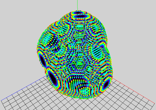
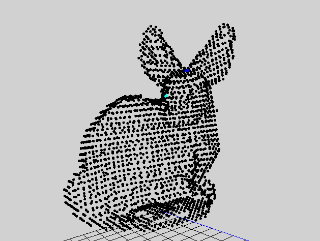
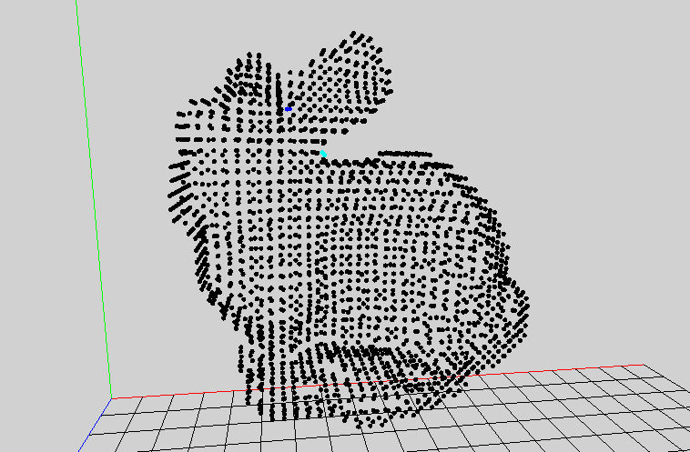
     Level Sets is a surface reconstruction technique that embeds a set of input points in a higher dimension to eliminate interface tracking. Taking the input points, lines, and surfaces, the algorithm computes the scalar distance function on a uniform three dimensional grid. Using the scalar distance function, you calculate the gradient of the distance function at all grid points. After these preprocessing steps, the algorithm creates an initial surface that is a bounding surface of the input set. This bounding surface can be any bounding surface, but in my implementation I chose to use the distance == epsilon point set as the initial surface.

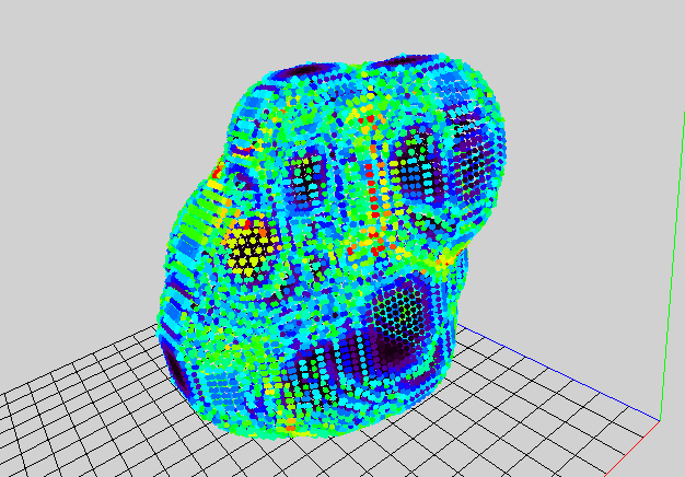
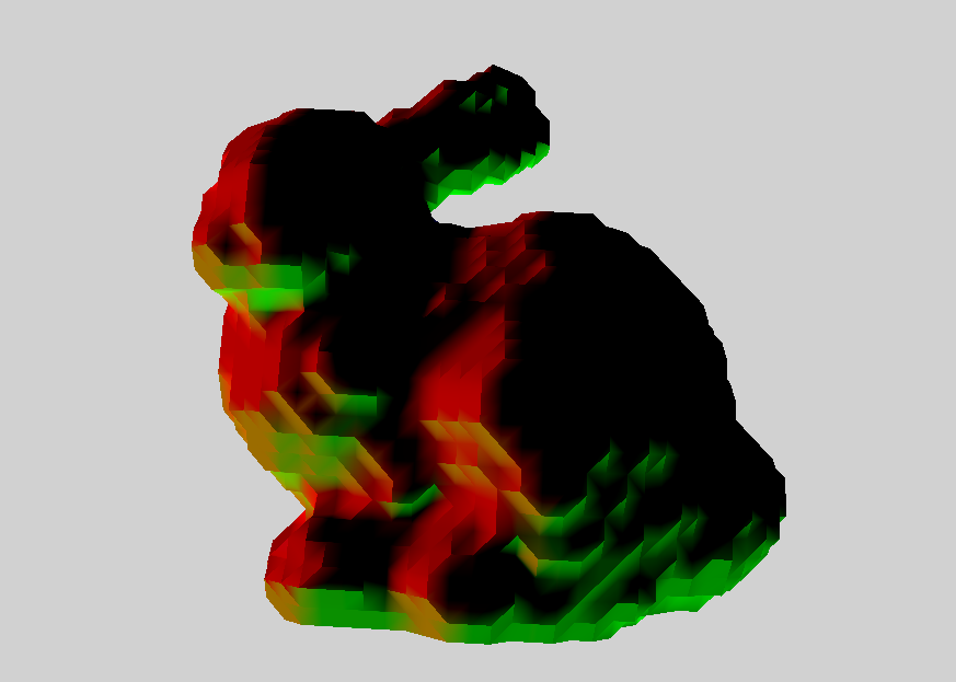
     Once we have our initial surface, the remaining portion of the algorithm iterates over the following steps until all points in the interface have reached the final surface:

  1. Calculate the signed distance function, phi, and normal field, N, in a narrow band around the current interface.
  2. Update the phi funtion using a gradient descent method. In practice, the update function TIME_STEP*dot(gradient, normal) works well.
  3. Extract the updated interface from the new phi function. This is done by finding all zero crossings in phi.

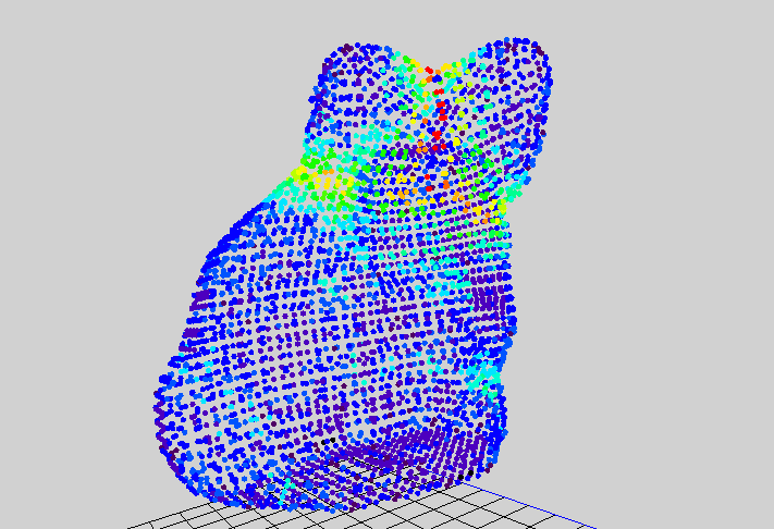
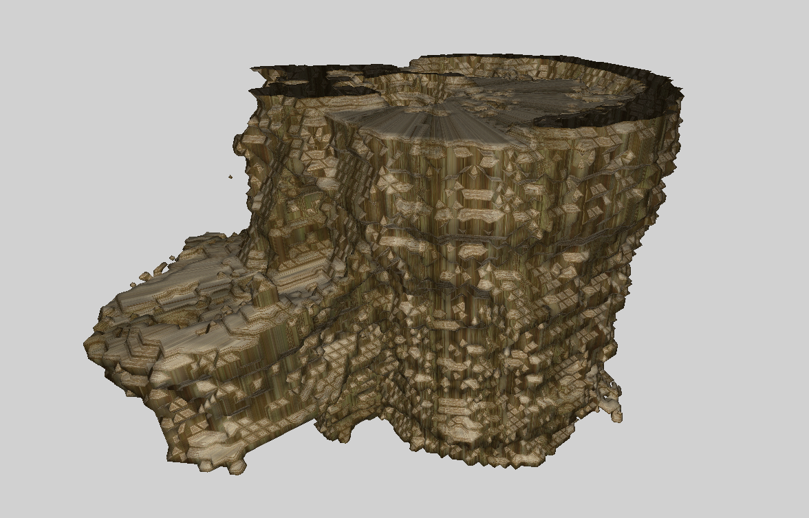
     Once the interface reaches the final surface, the interface can be used to create a signed distance function on the three dimensioanl grid. Using marching cubes, we can extract the zero isosurface from the volume to create a final mesh.