Kyle Haughey - CSC 572 Final Project - GPU Smoke Simulation
Email: khaughey {at} calpoly {dot} edu
Please email me with any comments or questions about this work. I would be happy to help you in any way I can!
Introduction
There is an ever-increasing need for more realism in today's movies and video games to immerse viewers and players in virtual worlds. Sometimes, artists can cause virtual characters to mimic behaviors observed in the real world. However, to achieve true realism, one must simulate the physics involved in underlying physical phenomena. Phenomena that are often simulated instead of directly animated include collisions, wind, water, and smoke.
Smoke!
This project investigated smoke simulation, and implemented a simulation based on solutions to the discrete Navier-Stokes equations. Because simulations are typically very computationally intensive, I thought that I could get more performance out of the GPU as compared to a CPU-only implementation. Therefore this project contains both CPU- and GPU-based smoke simulators.
Using the GPU to perform calculations is advantageous because the algorithm's calculations are independent of each other, and the GPU can perform many calculations simultaneously. The GPU is also optimized for vector and matrix operations, which are common when simulating physical phenomena in 2-dimensional or 3-dimensional space.
The GPU simulation achieves roughly 16x better performance than the CPU simulation, based on a simple framerate vs. resolution metric.
The Math
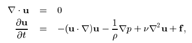
There are several methods used to simulate smoke and fluids in general, and this simulator uses the incompressible Navier-Stokes method. The Navier-Stokes equations were developed by Claude-Louis Navier and George Gabriel Stokes in the 19th century (working separately). The equations seen below are the Navier-Stokes equations with the added constraint of fluid incompressibility, where u is the fluid velocity, ρ is the fluid's density, p is the fluid pressure, ν is the fluid's kinematic viscosity, and f is the sum of external forces.
(Source: Stable Fluids)
Similar (in fact, nearly identical) equations govern the motion of particulate matter, such as smoke particles, that move around within the fluid.
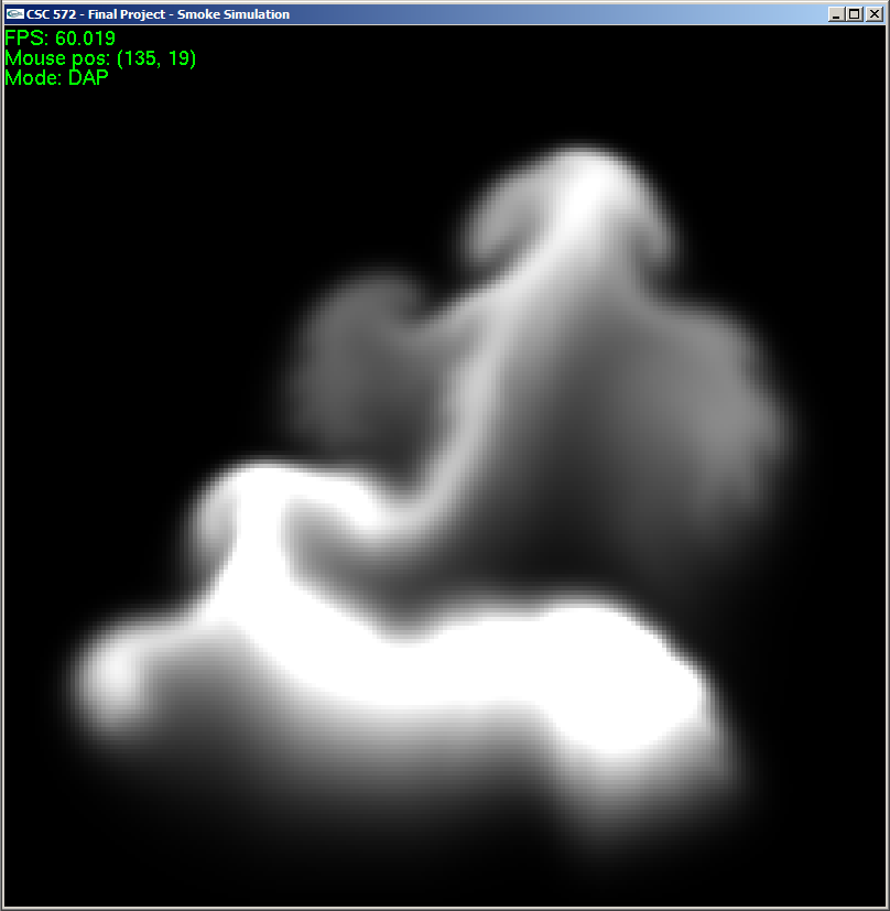
The fluid solver operates on discrete grid, where each grid cell has a velocity and smoke density.
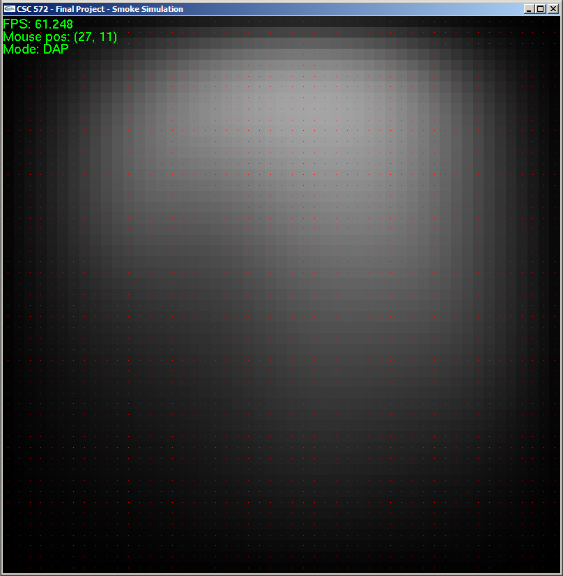
Grid cell centers (shown in red).
Velocity field (shown in yellow).
The solver works by finding a discrete solution to the above equations on the grid over some small timestep, and does so in six phases:
- Calculate forces - calculates buoyancy (smoke is warm, so it rises) and vorticity (small-scale swirl) forces for each grid cell (see references)
- Add forces - adds user-defined and calculated forces to the velocity in each cell
- Advection - moves velocities and densities along existing velocities
- Project - forces the velocity field to be conservative (divergence-free) by using the Helmholtz-Hodge Decomposition (see references)
- Diffuse - moves a portion of velocities and smoke densities to neighboring cells
- Project - same as before
The Simulator
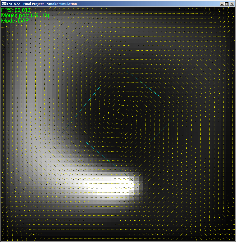
The simulator works in real-time, using the OS' native high-performance timer. Each frame, the simulator calculates how much time has elapsed since the previous frame and then simulates that amount of time. Users can add smoke at chosen locations as well as define their own forces (see "Running the Simulator" below).
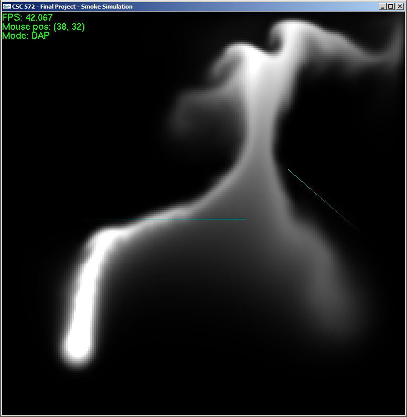
User-defined forces (shown in blue).
CPU Simulator
The CPU simulator uses simple 2D arrays of floats to hold values in the velocity and density grids, user sources, and user forces. It isn't very interesting :).
To display the smoke, the simulator renders a quad for every cell, setting the color to a grayscale value proportional to the smoke density in the cell.
GPU Simulator
The GPU simulator uses textures to hold the velocity and density grids, as well as user sources and forces and the results of several intermediate calculations.
The simulator uses 32-bit float textures as defined by the ARB_texture_float OpenGL extension. Vector and scalar grid values are stored in the textures' RGBA components; for example, the velocity and density fields are stored in a single texture: R -> velocityx, G -> velocityy, B -> velocityz, and A -> density.
Calculations are performed using fragment shaders. Current grid values and intermediate results are specified as input textures to the shader, and the EXT_framebuffer_object extension is used to allow the shader to render to an output texture. This texture is then fed into the next phase of the simulation.
Here is a diagram of the render path for the GPU simulation:
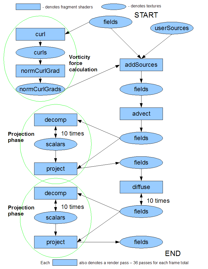
To get user input, the GPU simulator also has simple 2D arrays of floats that it uses to store user sources and user forces, just like the CPU simulator. At the beginning of each frame, the GPU simulator uses glTexImage2D() to turn the 2D arrays of floats into a texture that the shaders can use.
For display, the GPU simulator renders a single quad to the screen and uses yet another fragment shader to render the smoke color in proportion to the density in each cell.
Download
You can download and play with the simulator here.Since the fragment shaders are just plaintext files, you can play around with them too. They are in the shaders/ subfolder. Try tweaking some of the constants and see what happens!
Running the Simulator
Usage
smokeSim [-s] [res]
- -s: forces software mode; if not present, GPU will be used if available
- res: chooses resolution of the grid; must be an integer > 0
Controls
- ESC/Q - quit
- SPACE - toggle pause
- T - step the simulation by 0.1 seconds
- V - toggle rendering of velocity vectors
- C - toggle rendering of cell centers
- R - reset the simulation state, not including user forces
- F - toggle rendering of user forces
- S - toggle rendering of velocity vectors to scale (bigger vectors indicate higher velocities)
- A - toggle advection
- D - toggle diffusion
- P - toggle projection
- click and hold LMB - add smoke
- click and drag RMB - add user force
Status Information
- FPS - frames per second
- Mouse pos - the cell coordinates of the mouse cursor; (0, 0) is the bottom-left corner
- Mode - indicates whether [D]iffusion, [A]dvection, and [P]rojection are enabled
Known Issues
- If you right-click on the simulation area without dragging, you will create a singular force and will no longer be able to add smoke to the simulation. To fix this, simply press SHIFT + R to reset the forces.
- There is no way to remove user-defined forces one-by-one. To remove a force, you have to remove all of them with SHIFT + R.