The goal of this project was to implement a parallel version of photon mapping global illumination method. And it is my final project for the classes CPE 458 (Parallel Programming) and CPE 572 (Computer Graphics for Graduates) at California Polytechnic University.
Photon Mapping is a two pass global illumination (GI) method developed by Henrik Wann Jensen. The first pass will cast photons into the scene and the second will render the scene.
In the first pass, for each light source, you will shoot photons into the scene. Each photon has an initial power, which is the light power divided by the number of photons being emitted by that light source. The photon direction will be defined by the type of light that you are using, in example with a point light source you will shoot photons in a random direction. After defining the power and direction of each photon, you will use the ray casting algorithm to check for intersections between the photon rays and your objects. If the photon hit a diffuse surface you will classify and store that photon in that point with its current power. The photon classification will be direct illumination, if it is the first nearest hit for that photon, or indirect illumination, if that photon bounced and hit another surface, or shadow photon, if it is the first hit but not the nearest.
Once your photon hit a surface, you need to decide if they will bounce or not. To decide that you can use the Russian Roulette method, which basically you will pick a random value and compare with the surface diffuse and specular values. If the random value is greater than both the photon will be absorbed. Otherwise, the photon will bounce and its power should be scaled based on the material properties.
In the second pass, you will use the information stored in the photon maps to help the ray tracing. In this pass, you have to ray trace your scene and shade each pixel. There are four main things to render when you are using photon maps: Direct Illumination, Indirect Illumination, Reflective and Refractive Surfaces, and Caustics.
Direct Illumination is how that point is being illuminated by the light sources. With the photon map you will know based on the direct illumination and shadows photon stored. If the photons stored near that point are all of the direct illumination type, you will normally shade that pixel. If they are only shadow photons, you will shade that pixel in shadows. But if there is a mixture between both types, you will shoot shadow rays to the light source to get soft shadows. With this approach the number of shadow rays casted are reduced, because you only need to shoot them in the edge of each shadow.
Indirect Illumination is how that point is being illuminated based on how the light is interacting with the environment. This part will basically deal with the color bleeding. To render it you will use the indirect illumination photons to give information to the irradiance caching method.
Reflective and Refractive Surfaces are normally raytraced, because is hard to use photon maps to render them. The reason is that the color of those surfaces are based on the eye position, and during the first pass you are not considering the eye, just the light source. The probability of a photon hit the specular surface in the same angle that your eye is going to see it is very low.
Caustics are the effect produced by refractive surfaces. Using photon maps to render them is very easy and straightforward, because you only need to look up the values into the photon map and display them. With the N nearest photon you will use the Radiance Estimate to approximate the color on that point. Rendering caustics with normal ray tracing is hard and expensive, so you need more photons to be more precise with the radiance estimate. More the photon maps are dense more precise is the radiance estimate. Usually, the caustics photon map is generated separated, because they require more photons than usual.
Once that you render all four components your rendering step is complete. The photon map technique is very fast compared with raytracing, because it requires less rays and less spatial queries. It is the best known technique to render caustics, and provides full GI for your scene.
I implemented three parts from the whole photon mapping method.
For the photon casting I am using the ray casting approach. From my spot light source in the ceiling I shoot photons in the scene using random directions [1]. When the photon hit a diffuse surface, I store it in the photon map and use the russian roulette to get the new photon power and direction.
In the russian roulette I chose a new direction for the photon based on the material properties. If the photon is going to be reflected diffusely, I pick a random direction around the normal. If it is reflected specularly, I use the reflection vector as a new direction. The photon power scaling is described by Jensen in [1].
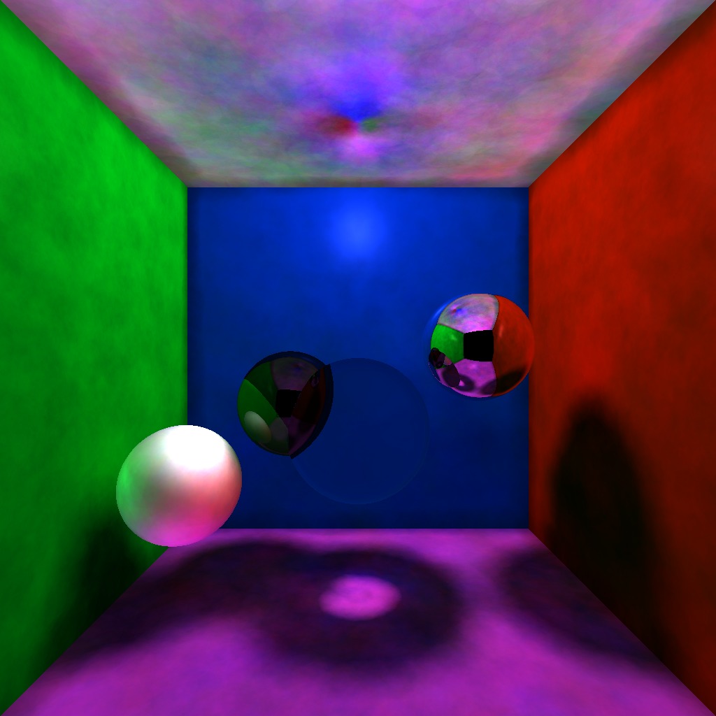
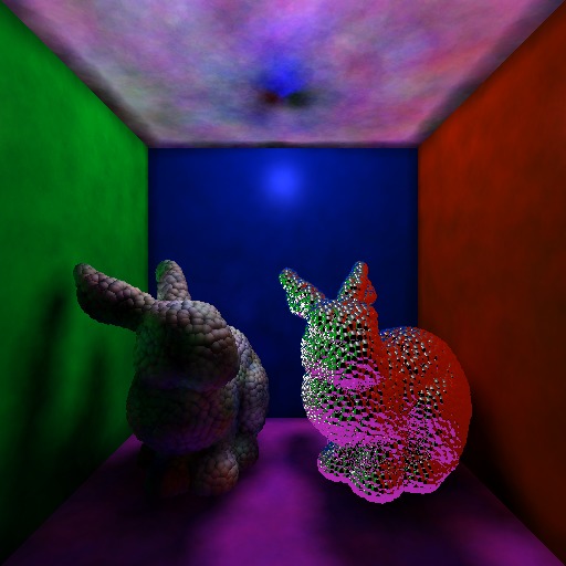
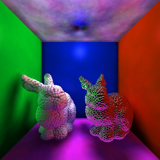
In the end of this pass I am generating one global photon map with all my photons. I tried two different approaches, generating one photon mapping (first image), and generating one global and one indirect illumination map (second image). As you can see, the with the two maps the color is bleeding excessively. But gives you a brighter scene.
The ray object intersection in this pass is parallelize to return all the objects which that ray intersects. With that I can classify the direct illumination and shadows photons more quickly. To implement that I used a parallel for to check the intersection between all the objects and a thread safe container to store the information.
To spatially organize my photons I am using a Left Balanced kd-Tree. The reason that I choose this data structure is that is very compact in memory, since you can use a flat tree. The flat tree is an array representation of a tree, where the left child is in 2i + 1 and the right child is in 2i + 2 (index starting at 0). It is very compact and fast, but to get the most compact space you need to left balance your tree. The left balancing guarantees that all leftmost leaves are occupied.
This is step is very hard to parallelize, because balancing a tree is a recursive problem and does not generate a fixed workload for your threads work on. Fortunately, it is also a very fast algorithm.
The radiance estimate is the heart of the rendering step. You are going to perform it at least once per pixel. Which is another reason to use a tree data structure. Because in the radiance estimate you are going to look up for N photons in the tree given a radius. With a balanced tree the search time is very efficient: N*log(N).
Parallelizing a search on a tree is very hard also, because of the same reason of parallelizing the tree construction. It gets even worse because the workload decreases quadratically. That is why I decided to not parallelize this step. But the rendering algorithm, which is a basic ray casting, is perfectly parallelizable. So, I put my effort in parallelizing it.
Parallelize a Ray Caster is pretty straight forward since each pixel is independent of the others. To do so I used a parallel for to iterate over the pixels.
When you are using photon mapping, there are several parameter that you need to use to get your images looking right. They are: Initial Photon Power, Number of photon gathered, and Radius of the N Nearest photons. The parameter that I used was respectivly 0.5, 100 and 0.25.
Each value for each parameter gives you a different image. If you initial power is too small, your scene is going to be darker. If you are no gathering enough photons you can end with black holes in your rendered image. If your radius is too large it will consume too much time to search for the photons, and if it is too small can create lots of false color bleeding and shadows.
Another parameter that you can tweak is the random direction that a photon can take after bouncing diffusely from a surface. This direction is based on the normal direction, you can tweak how much will vary from the normal. The color bleeding will be affected by this angle.
In this section I will analyze and discuss the result and progress that I had with my implementation. For this analysis I am using a i7 intel machine, with 2 physical cores and 4 logical. The perfect speed up should be around 2.5x.
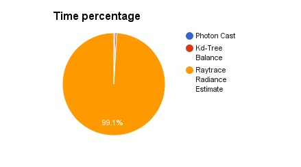
At first I time the 3 main parts of my implementation: photon casting, kd-tree balance, and rendering. As you can see below with the smallest scene the rendering time is 99% of the execution time. Which is why I started by parallelizing it.
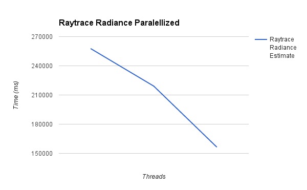
After the first approach, where I parallelized the Rendering step, I got 1.41x speedup for a small scene. My small scene has 9 objects, 1024x1024 in size, and 70000 photons. The graph below show the time for each number of threads (1, 2, and 4).
After that, I ran a profiling tool called Zoom in my code and I found that the radiance estimate was the most time consuming function. Which is expected, it is the heart of this method. The tool suggested to me too not use this method as a recursive function. Then I implemented a non recursive approach. With this approach I got slow down compared with the last version, the overall speed up with the non-recursive was 1.5x. The reason for that is that I am not optimizing this non-recursive function. When you use a recursive function and the flag -foptimize-sibling-calls, activated with optimization level 2 or higher, the compiler already implements a non-recursive version for you which is optimized. After figuring that out I reverted my changes for the last version.
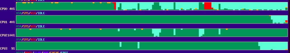
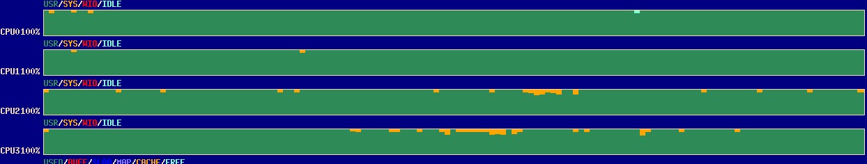
Another thing that I observed was the workload balance. After running the xosview program, I saw that my cores were being fully occupied. Then I changed the scheduling thread method from static to dynamic, which tries to keep all the cores busy. After this change I got a small speed up of 1.6x.
Static Scheduling
Dynamic Scheduling
The final result: It took 156 seconds to render the small scene and the large scene took 204 seconds. The large scene has 5012 objects, 100000 photons, 1024x1024 resolution. With the large scene I got 1.7x of speed up. You can see the images in the next section.
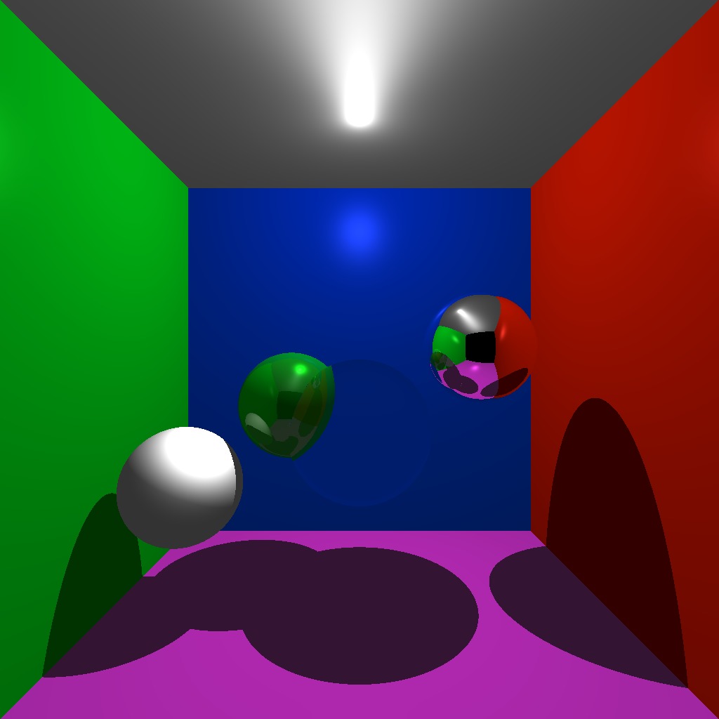
In this section I will be analyzing to main scenes that I selected. Both were rendered using my implementation. To render then I am using just the radiance estimate for all parts of the render equation, except for the reflective and refractive surfaces. I am also rendering caustics with the global photon map, I am not using a separate map, which is the why the caustics are so weak.
In this first scene, my small scene, you can see some color bleeding in the leftmost sphere. You also can see the weak caustics being casted from the glass sphere in the center. And the mirror sphere reflecting the scene in the right, and a slightly reflective sphere on the left behind the glass. The ray traced version is presented next.

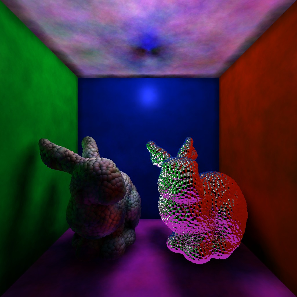
In the second scene, the large scene. I have two bunnies made of spheres, the rightmost is using the mirror material.
Photon Mapping is a very fast technique and gives very good results. But there are too many parameters to tweak to get the right result. Finding the perfect combination can give you some headache.
There is a lot of future work to do, that I couldn't implement due time issues. I will list some of them:
The whole project was developed and tested on a Ubuntu 14.04 with ICC 15.
To install and run this project you will need:
In order to install just follow the commands inside the project folder:
$ mkdir build
$ cd build
$ cmake ..
$ make
To run the project, run the photonmapping executable.
Author: Matheus de Sousa Faria matheus.sousa.faria@gmail.com