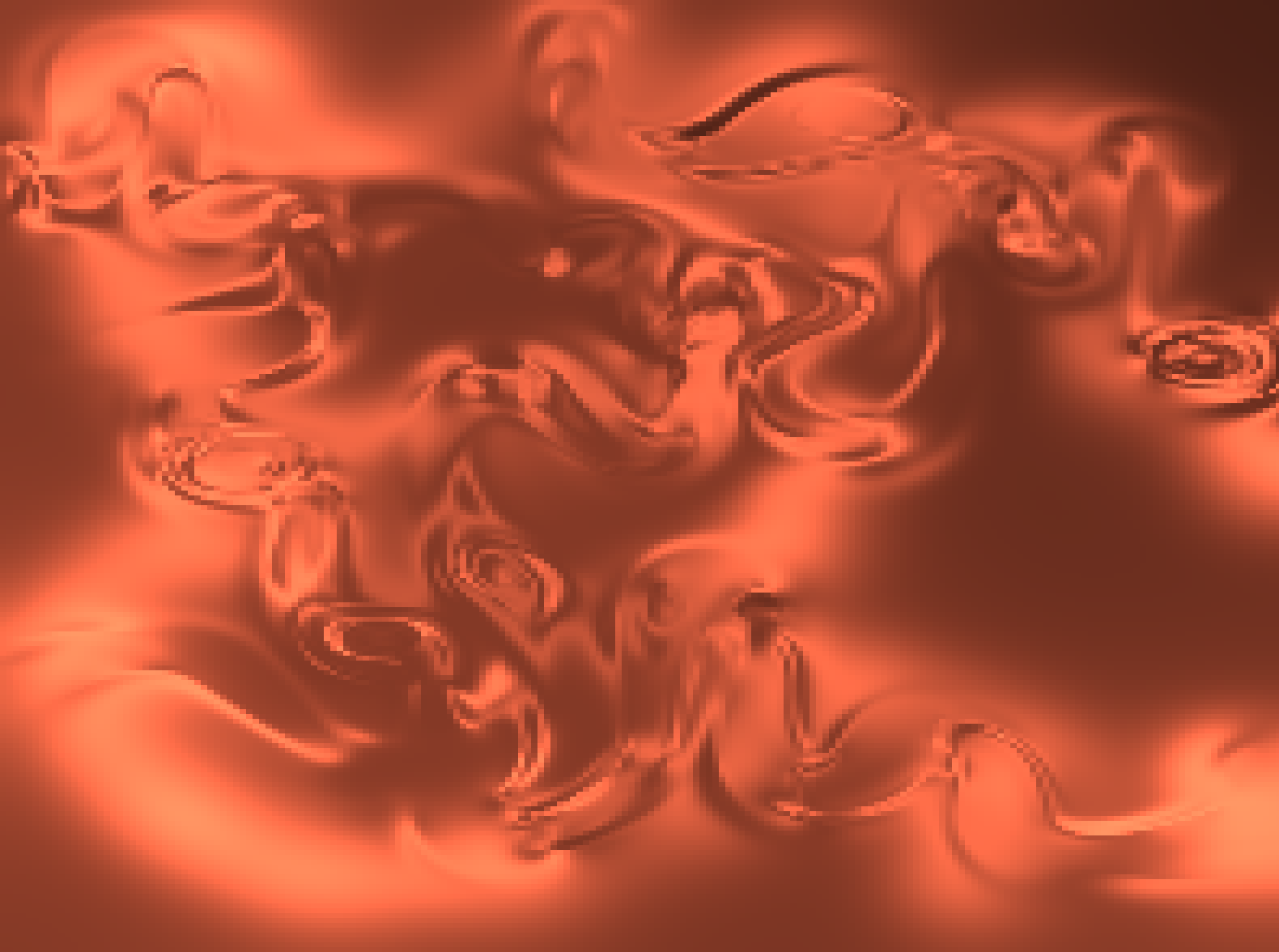


For this project I implemented a 2D Fluid Dynamics Solver based off Jos Stam's research paper Real Time Fluid Dynamics for Games. The paper explains how to simulate fluids and provides a C implementation of the solver. This implementation is based off of the Navier-Stokes equations which model the flow of fluids. One thing to note about the solver is that it is not an accurate representation of how fluids actually move in nature; rather it is an approximation that looks accurate and executes quickly—which is what we care about in Computer Graphics. Below you can find a demo of the simulation.
The Navier-Stokes equations tell us how a fluid will move over a single time step. First, we split a region of space into a 2D grid. We then create a density field, where each value in the density field represents the amount of fluid present in that grid cell. We also create a velocity field, where each cell contains an x and y component representing the forces acting upon that cell. Each time step, we start with an initial density field and velocity field. We then compute a new velocity field, and new density field. This newly computed density field tells us how much fluid is present in each grid cell.
Every frame we collect user input (for both density and velocity), calculate the velocity field, calculate the density field, and then draw the density.
Since we want a way to interact with our program, we allow the user to inject density into the grid and add forces to the grid. We allow the user to inject density by pressing the ‘d’ key while dragging the mouse across the screen. Every grid cell the mouse drags over will then receive some density. We also allow the user to add forces into the scene by pressing ‘f’ and dragging the mouse across the screen. The x and y component of the force are computed by the mouse movement. Every single frame, we collect the user input (sometimes there may be none), and store this input in three different arrays: densityInput, velocityXInput, and velocityYInput. These three arrays are then passed into the solver code and used to calculate the final density value.
According to the Navier-Stokes equations, the velocity field is computed via user inputted forces, viscous diffusion, and self-advection. The user-inputted forces are simply received via the user’s input. Viscous diffusion is what makes the simulation look like either water or oil. Self-advection may sound confusing, but simply means that the velocity field moves along itself. The result of this step is a newly computed velocity field.
According to the Navier-Stokes equations, a density field can be computed from a velocity field, diffusion, and various sources. We receive the velocity field as an input, and use this velocity field to calculate the flow of the fluid. Diffusion simply means that density will spread across the grid cells. This is computed for each cell by calculating a net density: the amount of density present after each cell gains some density from it’s four direct neighbors, and then loses some density to those same four neighbors. The various sources represent any density in the scene that is present before any computations have been made. This initial density can be supplied in two ways: user input or hard coded.
After calculating the new density field, we have an updated density field that represents the amount of fluid present in every single cell in the grid. We then use this density field to update the density values for each cell and draw them.
For my implemenation, the solver computations were performed on the CPU and then the updated density values were passed to GPU every frame. Since my implementation was in 2D, I decided to use the Z component for each vertex to store the density value of the grid that the vertex belonged to. I used indexed based buffering, so the amount of vertices I had was (gridSize + 1)*(gridSize + 1). Then, every frame I updated the Z component of the vertex to the corresponding density value from the density field. I then sent the entire list of vertices to the shaders to render the scene. Since the vertices are static, I probably could have sent only the density values to the shaders to reduce the amount of data passing from the CPU to the GPU. But as I’ll talk about in the results section, the main bottle neck of the program was not data transfer between the CPU and GPU, but rather the grid size.
My main conclusion from this project is that fluid simulations are computationally expensive and there is a tradeoff between accuracy and performance. There are two main factors that influence the performance of the solver: the grid size and the number of iterations over the grid per frame.
Grid size affects the performance of your program. The larger your grid size, the slower your program runs. You can see the effects of different grid sizes in the chart and videos below.
| Grid Size | Average Frame Rate |
| 50 x 50 | 60 frames per sec |
| 150 x 150 | 30 frames per sec |
| 200 x 200 | 15 frames per sec |
| 400 x 400 | 3 frames per sec |
| 1000 x 1000 | 3.5 seconds per frame |
Lower grid sizes run faster, but have lower resolution. Higher grid sizes have higher resolution, but run much more slowly. You can see in the videos belows the difference in resolution and runtime for each grid size. (For all videos the width of the OpenGl window was 800 pixels, and the height was 600 pixels)
Note: I didn't include a video of the 1000x1000 grid size because it was really, really slow.
The code for the solver that Stam provided performs 110 iterations over the entire grid every single frame. For each function that the solver calls, I computed the number grid iterations by multiplying the number of times that function was called (per frame) by the number of grid iterations each single call performs. You can see the results below.
| Function | # of times called per frame | # of grid iterations per fuction call | Total # of grid iterations per frame |
| Diffuse() | 3 | 20 | 60 |
| Project() | 2 | 22 | 44 |
| Add Source() | 3 | 1 | 3 |
| Advect() | 3 | 1 | 3 |
Unfortunately, grid iterations are really expensive. In 2D, each grid iteration costs GridSize * GridSize single loop iterations. In 3D, each grid (or cube) iteration costs GridSize * GridSize * GridSize single loop iterations. Below, you can find a chart that shows the number of loop iterations per frame for Stam’s solver in both 2D and 3D. (Note: I am ignoring the set_bnd function which is called X times per frame and includes a loop that goes from 0 to GridSize)
| Grid Size | Loop iterations per frame (2D) | Loop iterations per frame (3D) |
| 50 | 275,000 | 13,750,000 |
| 150 | 2,475,000 | 371,250,000 |
| 400 | 17,600,000 | 7,040,000,000 |
| 1000 | 110,123,012 | 112,000,000,000 |
As you can see, these computations can get really expensive really fast. One way to improve the speed of the solver (without reducing the grid size), would be to reduce the amount of grid iterations per frame. Recall from above that the functions diffuse and project both perform a high amount of grid iterations per function call. I decided to reduce the amount of grid iterations in each of these functions in order to increase the speed of the solver. In diffuse, I changed the amount of grid iterations from 20 to 2. In project, I changed the number of grid iterations from 22 to 2. Before, diffuse performed 60 grid iteration per frame and project performed 44 grid iterations per frame. But with my changes, diffuse now performs 6 grid iterations per frame, and project performs 4 grid iterations per frame. Overall, the total number of grid iterations dropped from 110 to 16. Below you can find two videos that show the simulation before and after my changes; the one on the left shows before, the one on the right shows after. Both these videos use a grid size of 200 x 200.
As you can see from the videos, there is a tradeoff between visual accuracy and speed. The more realistic (and better looking) you want your simulation to be, the slower it will run. The faster your program runs, the less accurate it will be.
The research paper I used was written by Jos Stam and can be found here.