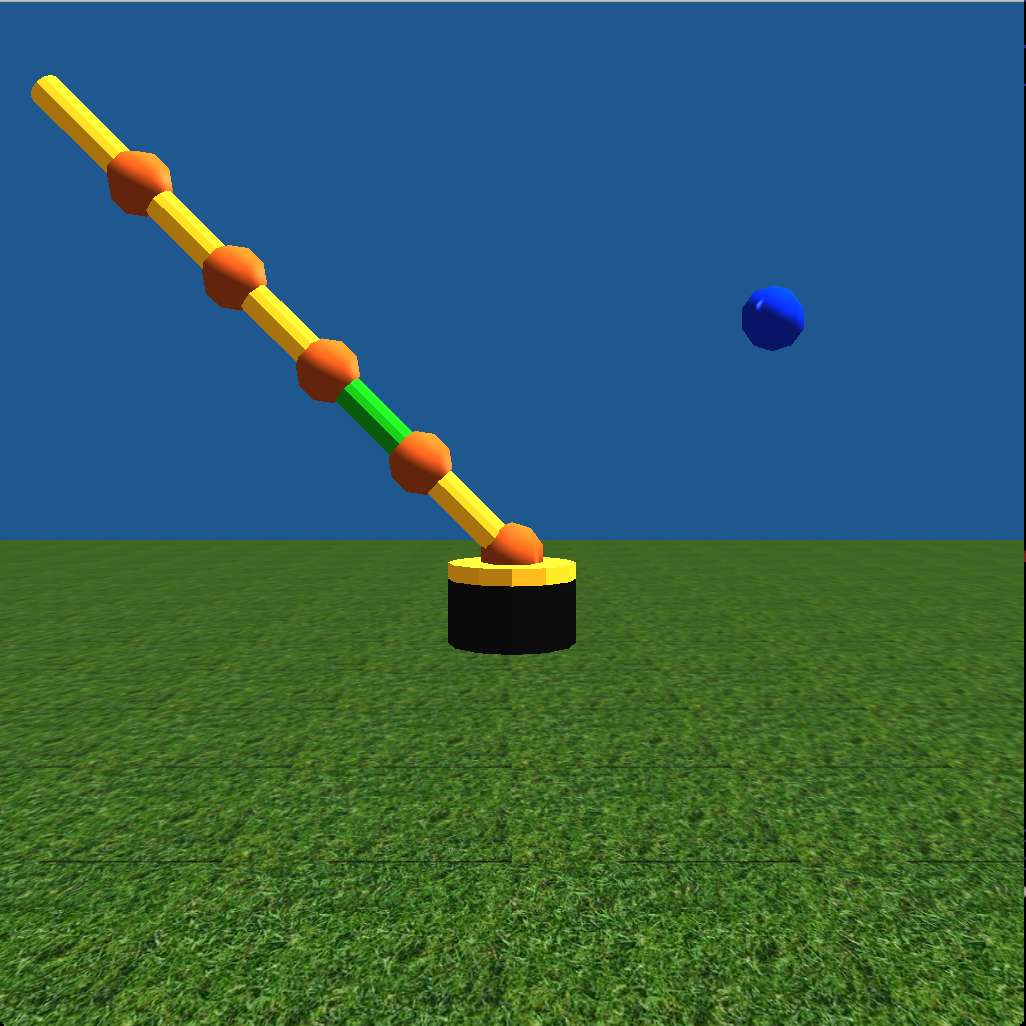
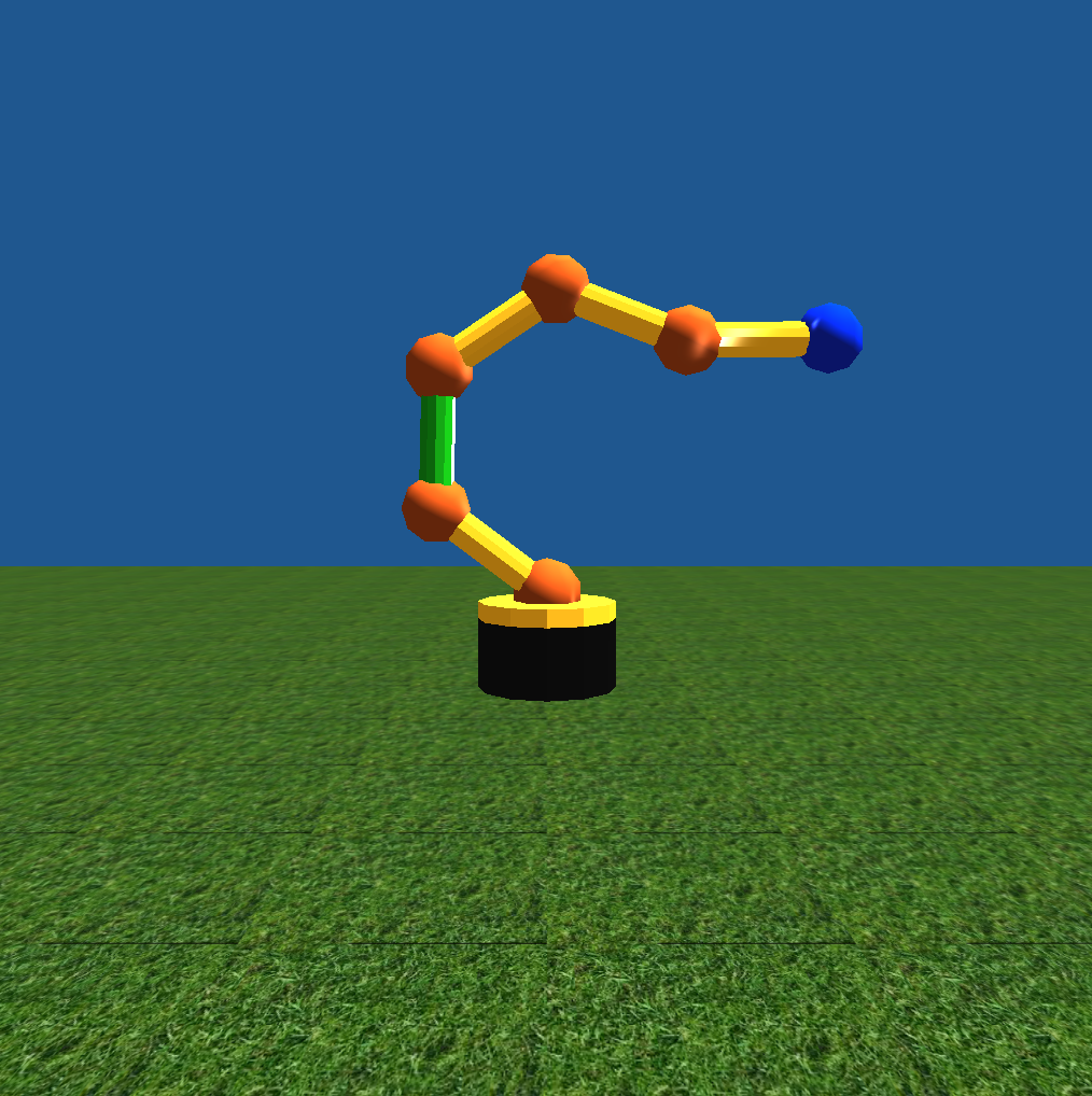
For my final project in CSC 572, I decided to solve an inverse kinematics problem. As input, I took a number that would represent the number of components that made up a robot arm. This arm was on top of a rotating lazy susan allowing it to reach anywhere in 3D space within the length of the arm since the components were only able to rotate on one axis. An example of an arm with five components is shown below. (The blue ball in the picture represents the desired end location of the end of the arm.)
I tried a couple of different methods for solving this problem.
First, I went about it without much to go off of besides my own mathematical knowledge. I tried to create an equation that would use variables for every angle and solve for the final location. Then, I would be able to plug in the desired location for the final location. Of course, there are too many variables for this to work. As a result, I limited every angle besides the first one to be equal. This meant that if you created a line from the base of the arm to the desired location, the angle in which the first component deviated from the line (let’s call it theta) would be equal to the twice the sum of all of the other angles (let’s call each one phi). In other words:
Although there weren’t too many variables in this equation, it was too difficult of an equation to solve with my knowledge of cosines and identities even when trying to look it up. For a while, I tried to find more constraints that would make it solvable, but I couldn’t find one that worked.
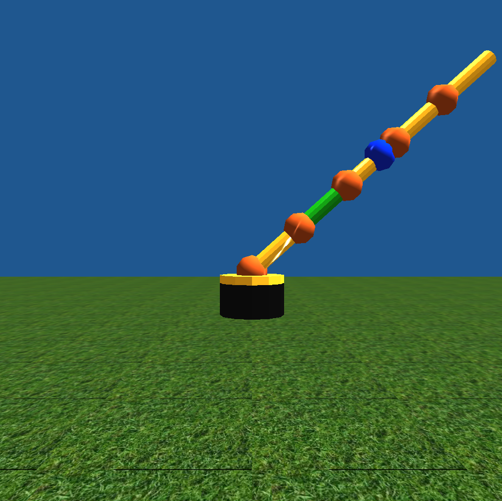
Next, I decided to take an iterative approach. This involved calculating the angle of the lazy susan in order to allow the components to rotate along an axis, which would allow them to reach the desired point (the blue ball). Next, it would overshoot the point by creating a vector from the base to the desired point and calculate the first angle from there. This would look something like the arm below:
Next, the arm would iteratively “back off” of the vector calculated from the base to the desired point. It would increase the angle of the first component while decreasing the angles of every component afterwards using the same equation as above:
where theta is the angle between the desired vector and the first component and phi is every subsequent component’s angle relative to the component before. As a result, with every iteration, the end-effector of the arm (the very end of the arm) always lands on the vector between the base and the desired point.
It then finds the actual location of the end-effector using a matrix stack and hierarchical modeling for each component to be based on the last ones. Finally, it calculates the distance between the end-effector and the desired location to find the error. It then continues the iteration until the error is no longer getting smaller and is getting larger instead.
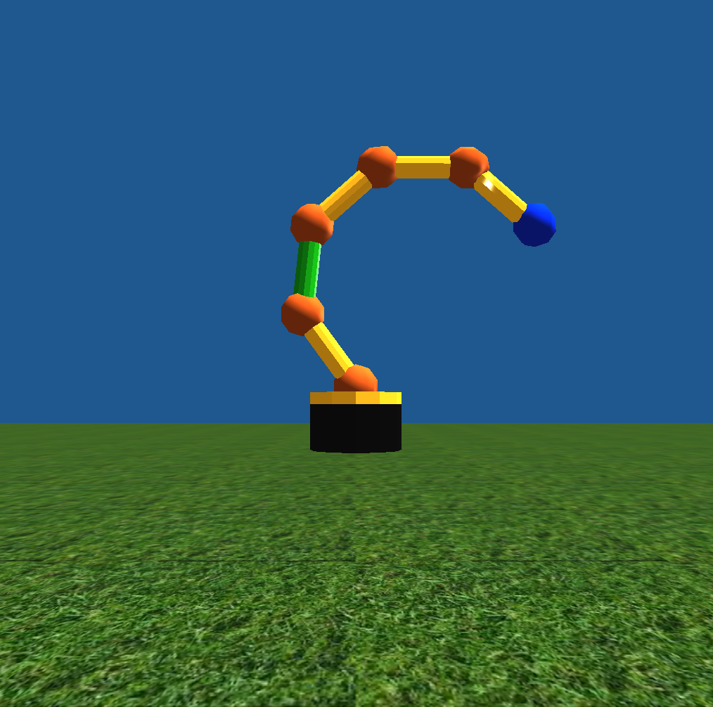
By the end of the algorithm, it looks like:
Although this method was successful, I really wanted to create an exact algorithm rather than an iterative one.
Next, I made another attempt to get an exact algorithm using an algorithm from Rick Parent's textbook (cited below). This involved using a Jacobian matrix and inverting it to solve for the change of angles. Given the points of the current positions of each elbow along the arm, you can create the Jacobian matrix. Along the rows of the matrix are the differences in space of the end-effector from each elbow of the arm. Along the columns of the matrix are the different components of the vector (x, y, and z).
The next step of the algorithm is to invert the Jacobian matrix and multiply it by the vector representing the difference in space from the end-effector to the desired point. Unfortunately, it’s not an easy task to invert the Jacobian matrix. After a lot of trial and error with this method, we realized that the matrix was never going to be invertable. This is because the change in the z component is always 0 (as we are solving a 2D problem after rotating the lazy susan). Since one of the zeros is on the diagonal, the matrix was never going to be invertible. We then realized that there were others ways to estimate the inverse of the Jacobian matrix. With very little time left over, I was not able to compute the “pseudo-inverse” of the Jacobian algorithm. I did try the first solution suggested by the book. It involved creating a two-by-three matrix out of the first two rows of the Jacobian matrix (the rows with the x and y component, and excluding the z component row). You then multiplied it by its transpose (a three-by-two matrix). You’re left with a three-by-three matrix, which you would hope is invertible. Unfortunately, although it did create a matrix without any zeros, I did not have enough time to find values that did allow this method of inverting to work. There are other ways to attempt the inverse as well, and eventually it resorts to an iterative method as well. I hope that in the future, I will be able to implement this method to find an exact solution and allowing the angles to vary independently.
After implementing the iterative algorithm (Method 2), I decided to take it a step forward. Thinking about the purpose of this robot arm, which is to eventually accomplish a task, I thought that it would often be important to specify the direction that the robot arm reaches the desired point from. For example, if the arm is trying to grab a ball from a counter, it can’t grab it from below the table, and it probably won’t be very successful at grabbing it if it comes from the side. Thus, the user would want to specify that it must grab the ball from above. I added the ability to specify the directional vector that the robot arm approaches the desired point.
As an example, below depicts the arm approaching the desired point from the vector (0, -1), or straight down.
This addition to the algorithm meant finding the desired position of the second-to-last component. This wasn’t too difficult as it merely meant translating the desired position into its desired 2D coordinates and subtracting the normalized vector that it was meant to approach from times the actual size of the last component.
Using the position of the second-to-last component, I ran the iterative algorithm using that as the desired component and subtracted one from the number of components. From there, I knew all of the desired angles apart from the last one.
Saving the vector that went from the third-to-last component to the second-to-last component, I was able to calculate the last vector’s angle. That angle between that vector and the desired approaching vector was the angle that the last component needed to be rotated at.
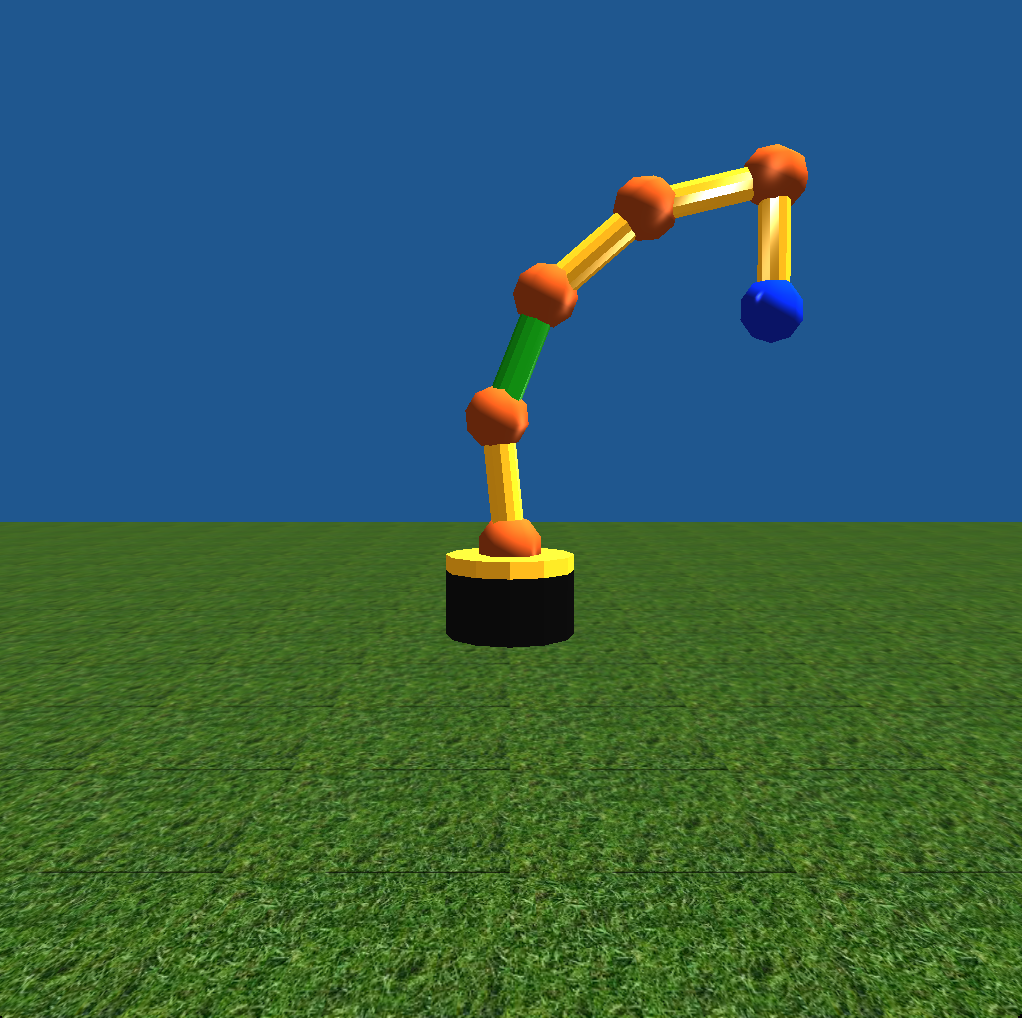
Below you can see another use of this algorithm, which takes in (1, 0) as its desired approaching vector:
Finally, I had an algorithm that would allow you to reach the desired point from any angle.